integrating symbolic and numeric techniques in atomic physics

FEATURE ARTICLE

INTEGRATING SYMBOLIC AND NUMERIC TECHNIQUES IN ATOMIC PHYSICS This article describes ISNAP, a program for calculating atomic properties that uses an integrated symbolic and numerical approach for arbitrary excitations from closed-shell atoms. This program generates transition matrix elements and energy formulas up to third-order perturbation via the symbolic programming language Mathematica.

I

nterest in the many-electron properties of atomic systems has focused attention on many-body perturbation theory (MBPT) techniques, which provide a powerful and systematic method for calculating atomic properties (such as energies and transition rates) with systematically increasing precision. However, the number of perturbation terms increases rapidly with the complexity of each order of MBPT, reaching several thousand in third order for relatively simple problems. Researchers commonly use the Feynman diagrammatic procedure1 to reduce the terms to a smaller set, which they then evaluate numerically with problem-specific programs.2 The visual nature of the diagrams corresponding to the terms tends to make this reduction process intuitive. However, in higher-order MBPT terms,

1521-9615/01/$10.00 © 2001 IEEE

WARREN F. PERGER AND MIN XIA Michigan Technological University

KEN FLURCHICK Ohio Supercomputer Center

MOHAMMAD I. BHATTI University of Texas Pan American

22

drawing the diagrams requires a high degree of proficiency to avoid omitting terms and introducing errors, such as with term signs and labels.3 Underlying the diagrammatic approach is Wick’s theorem,4 which we express using second-quantized forms for the interaction Hamiltonian as well as for the initial and final states. The representation of the operators—that is, the combination of a creation and an annihilation operator—is formally equivalent to the combination of two free lines in a corresponding Feynman (or Goldstone) graph. As with the diagrammatic approach, using Wick’s theorem to obtain the MBPT terms is tedious and error-prone when done by hand, suggesting the need for a different approach, such as using a computer-algebra system to perform the necessary algebraic manipulations on Wick’s theorem. To date, there are a few programs to perform the algebraic reductions using Reduce5 and Mathematica.6–9 However, this reduction is just the first step toward performing a calculation capable of being compared with experiment; we must then reduce these many-body formulas for energies and transition matrix elements using the lengthy but straightforward angular reduction. Finally, we must numerically evaluate these reduced terms. The procedure to date has been to write separate numerical programs for each expression.

COMPUTING IN SCIENCE & ENGINEERING

Wick’s Theorem and the atomic problem This article describes ISNAP (Integrated Symbolic/Numeric Atomic Physics), an integrated suite of programs capable of performing all these steps automatically and producing numerical results for both energies and transition matrix elements, for open-shell systems and multiconfiguration atomic states. The user supplies a minimum input set (the number of particles and holes, atomic number, and so on). A suite of programs written in Mathematica 10 generates error-free MBPT terms for nonrelativistic or relativistic atomic systems, performs the angular reduction using an external Fortran program, Kentaro,11 and then numerically evaluates the resulting expressions using MathLink and C to access efficient, optimized, pre-compiled Fortran programs for numerical evaluation. We have carefully tested the programs described here against published results for the expressions for the 1-particle, 0-hole case,5 the 1-particle, 1-hole case,12 and the 2-particle, 0hole case13 and numerical results for the 1-particle, 0-hole case for atoms ranging from lithium to cesium.2 Throughout, we have made maximum use of existing software, such as Kentaro and the GRASP92 programs.14 We have written Mathematica functions capable of reuse for all orders in perturbation theory that never require writing any problem-specific code—thereby reducing the opportunity for introducing errors. Most significantly, the program described here seamlessly uses various programming languages, taking maximum advantage of the attributes of each. It employs Mathematica where lists and symbolic substitution are required; existing, optimized, Fortran programs where they are best suited; and MathLink to bridge the components. This approach allows the nonspecialist in MBPT to access previously inaccessible calculations of atomic properties. Figure 1 provides an overview of the entire process. It combines the results of the Wicks Thm program with numerical codes to compute a wide range of atomic properties, but it first performs an angular reduction on each MBPT formula. The user may also accomplish the angular reduction procedure, for nonrelativistic and relativistic cases, using a graphical procedure;3 we have opted to use Kentaro11 and have adapted it for this purpose by writing an

JANUARY/FEBRUARY 2001

Input data Number of particles, holes, and many body perpetuation theory order

WicksThm Mathematica program to calculate MBPT terms using Wick’s theorem

LaTeX output

WTtoTeX Formats MBPT

Kentaro

terms in LaTeX

Program to perform angular reduction

Prepares data for Kentaro; formats results in LaTeX

LaTeX output

evaluate Calculation of atomic properties, i.e., transition matrix, elements and energies.

MathLink

Basis set program to calculate relativistic atomic orbitals

MathLink

FORTRAN program to calculate RL (abcd)

Figure 1. A schematic illustration of ISNAP (Integrated Symbolic/ Numeric Atomic Physics), the suite of programs for an integrated symbolic–numeric approach for calculating atomic properties.

interfacing program, WTtoTeX. Finally, to calculate atomic properties, a separate program, Evaluate ML, organizes the output of WTtoTeX, creates the appropriate numerical sums, reads an atomic single-particle orbitals numerical basis set, and calculates the relevant numerical quantity.

23

MBPT formalism and second quantization In order to understand how we can use a computer–algebra system to solve the many-body problem, we must first show how specifying electron–electron interactions with “Second quantization” exploits the step-by-step nature of MBPT. The Coulomb interactions between electrons make the atomic problem more complex; therefore, an There are a large exact solution to the Schrödinger equation is not number of terms that achievable for complex atoms. However, by assuming each will cancel out electron moves independently in a central potential V(r) that automatically in the incorporates the effect of other electrons, we can make perturbation a reasonable zeroth-order approximation for the manyexpansion. electron system. In this approximation, we can split the Hamiltonian for the system (H) into two parts, a model Hamiltonian (H0) and a perturbation interaction V: H = H0 + V,

(1)

Let u(ri) be the model potential (which is often chosen to be the Hartree-Fock VHF(r) potential). By adding it to the first term of Equation 1 and subtracting it from the second, we can write: H0 =

N

N

i =1

i =1

∑ h(ri ) + ∑ u(ri ) N

V=−

∑ i =1

N

u(ri ) +

∑ i< j

e2 rij

(2)

(3)

systems, which makes the perturbation series converge rapidly. Additionally, there are a large number of terms that will cancel out automatically in the perturbation expansion, thereby reducing the number of formula terms to be manipulated and, ultimately, numerically evaluated. We can derive the MBPT formulas for particlehole excited states of closed-shell atoms using the second-quantized form of Rayleigh–Schrödinger perturbation theory. We can express the zeroth-order Hamiltonian H0 and the interaction V in the second-quantized form as H0 =

∑ ∈w aw† aw

where a†w and aw are the creation and annihilation operators, respectively, for state w. Using the HF potential as the model potential, the perturbation interaction in the second-quantized form is V=

∑

r r h(ri ) = cα ⋅ p + βmc 2 + Vnuc (ri )

(4)

where h(ri) is a single-particle Dirac Hamiltonian for an electron moving in a nuclear Coulomb potential Vnuc(ri). We select the Hartree–Fock (HF) potential for the model potential u(ri), because it is a reasonable approximation to the exact solution for many-electron

24

∑

1 gwxyz aw† a †x az a y − w u x aw† a x 2 w , x , y, z w, x

(6)

where the two-particle Coulomb g-functions, gwxyz, are defined by gwxyz ≡ α

∫

d 3rd 3r' φ w† (r )φ x† (r' )φ y (r )φ z (r' ) r r r − r'

(7)

and φ(r) are the single-particle basis functions. We can express the HF potential in terms of the g-functions as

w u x ≡ (VHF ) wx = =

For the case of a relativistic Hamiltonian, h(ri) is given by

(5)

w

∑ g˜ wαxα

∑ (gwαxα − gwααx ) α

(8)

α

where g~ consists of direct and exchange terms. In the following sections of this article, the labels α, β, γ, ... denote core orbitals (including the hole orbitals), the labels a, b, c, ... denote virtual orbitals (including the particle orbitals), and the labels w, x, y, ... denote indices for sums over either set of orbitals. A generalized particle-hole creation–annihilation operator, called the generalized state operator (GSO), is defined as

COMPUTING IN SCIENCE & ENGINEERING

OHP ≡ aa† ab† ...aα aβ

E(2) = 〈0|V|1〉

(9)

where P represents the set of particle labels, and H represents the set of hole labels. As an example, for the 1-particle 0-hole case, the GSO given in Equation 9 reduces to the simple form O P = a † , where a = 2s is a particle outside the closed core 1s2 for lithium. The application of the zeroth-order Hamiltonian H0 onto the model-space ket |0〉 yields (H0 – E(0))|0〉 = 0

(15)

where |1〉 is the first-order wavefunction obtained by solving the first-order MBPT equation |1〉 = (H0 – E(0))–1(E(1) – V)|0〉

(16)

where |0〉 is the zeroth-order wavefunction. We can evaluate the third-order energy expressions in either of two ways:16 3) E (3) = 1V 1 − E (1) 1 | 1 = E1(V3)1 + E (folded

(10)

(17)

where where O is for operator, P is for particle, H is for hole, and the zeroth-order wavefunction with specified total angular momentum is 0 ≡ 0 PH

and

= F[ P | H ]

OHP

(11)

0 core

3) (1) E (folded ≡ −( E (1) − Ecore ) 1|1

where F[P|H] is the appropriate angular Clebsch–Gordon coefficient with appropriate normalization factor and |0 core〉 is the HartreeFock closed core. As an example, the zeroth-order wavefunction for lithium will be |0〉 = a†2s|0core 〉. We can find the zeroth-order energy by applying the conjugate (bra) of Equation 9 to Equation 10: E (0) =

∑ ∈i + ∑

i = core

i = particles

∈i −

∑

∈i

i = holes

(12)

Using the HF model potential, V is simplified to a second-quantized, normal-ordered form (that is, all core creation operators appear to the right of all core annihilation operators, and all virtual creation operators appear to the left of all virtual annihilation operators) as V=

(1) E1V1 ≡ 1 | V − Ecore |1

∑

∑

1 1 gwxyz : aw† a †x az a y : − g˜ 2 w , x , y, z 2 α , β αβαβ

(13)

where the colons are a notation to indicate normal ordering.3

The MBPT expressions for first- and secondorder energies are given by E(1) = 〈0|V|0〉

JANUARY/FEBRUARY 2001

or (18)

E(3) = 〈0|V|2〉

where |2〉 is the second-order wavefunction. We programmed both expressions in Equations 17 and 18, then had Mathematica This use of the sort the lists, verifying termby-term comparisons for software to test itself cases (such as the 2-particle, 0-hole case), where the proproved helpful for liferation of terms makes the comparison laborious. This eliminating use of the software to test itself proved helpful for elimiprogramming errors. nating programming errors. To illustrate the use of ISNAP for a specific atomic problem, the expressions for the first- and second-order energies E(1) and E(2) for the 1-particle, 0-hole case, exactly as produced (in LaTeX form) by the program, are   1 (1) = Fb Fa  − δ ba Ecore g˜αβαβ    2   αβ

∑

Energy expressions

(14)

,

(1) Eval =0

(19)

(20)

25

β

A

β

c

Transition matrix element formulas

d

We develop the transition matrix elements as we did the energy expressions, order by order. We give the first-, second-, and a few terms from third-order for the 1-particle, 0-hole case for illustration, as written by WTtoTeX:

=

α

a

b

α

a

c

b

B

d

(a) β

δ αβ

δac

b

+ d

c +

α

–

d

δ ab

δ ab

δab

c

α d

d

(d)

β

+

δac (e)

δab

∑



∑ ∈acbαac− ∈cbαα  (23) g˜

T

cα

and  Tcγ gαβaγ g˜ bcαβ T (3) = Fb Fa  +   cαβγ (∈bc − ∈aγ )(∈bc − ∈αβ )

∑

+

Tcα g˜

g˜



∑ (∈bc − ∈aαbβ)(ad∈cdcdαβ− ∈αβ ) + ...

c

where T represents the matrix elements between different parity states.

d

Wick’s theorem reduction At the heart of our approach is the use of Wick’s theorem:4

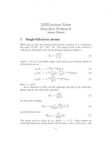
Figure 2. Example of the Wick’s theorem contraction process using diagrams.

} AB = {AB} + {AB}

E (2)

 gαβac g˜ bcαβ = Fb Fa  +   cαβ ∈bc − ∈αβ

∑

gαβcd g˜ cdαβ gbαcd g˜ cdaα  1 − δ ba −  ∈ − ∈ ∈ − ∈aα  2 αβ cdαβ cd cdα cd

∑

∑

(21)

Owing to the length of the third-order energy expression, E(3), we give only a few terms in Equation 22 that illustrate the method here.  g˜αγcd g˜ dβaγ g˜ bcαβ E1(V3)1 = Fb Fa  −2   cdαβγ (∈αγ − ∈cd )(∈bc − ∈αβ )

∑

−

∑

cdαβγ

∑

for the algebraic reduction of terms, where {AB} is} the normal-ordered product of A and B, and {AB} is defined as the sum of all the normal-ordered terms with single, double, and so forth contractions possible between operators A and B. As an example that illustrates the connection between the diagrammatic approach and the algebra of Wick’s theorem, consider the product of two operators A and B, where A = aα† a , B = aα† aβ a † a , and the labels conform to the convention described earlier. The application of Wick’s theorem, using the WicksThm program, yields:

+δ αβ ab† ac† aa ad − δ αβ δ ac ab† ad

(∈αγ − ∈cd )(∈cd − ∈αβ )  gγδcd gαβγδ g˜ cdαβ  (∈γδ − ∈cd )(∈cd − ∈αβ ) 

(25)

AB = {aα† aa ab† aβ ac† ad } + δ ac {aα† ab† aβ ad }

gαγcd g˜ bβaγ g˜ cdαβ

1 + δ ba 2 cdαβγδ

26

(24)

cdαβ

+ (f)

 Tcα g˜ bcaα T (2) = Fb Fa  − −  cα ∈bc − ∈aα

a

(c)

(b) b

b

+δ ab {aα† aβ ac† ad } + δ abδ αβ ac† ad

(26)

(22) Figure 2 shows the diagrams corresponding to these six terms.

COMPUTING IN SCIENCE & ENGINEERING

For this case, we see how the external lines of the diagram fragments A and B are joined to form the product of A and B. In (a) no lines are joined, giving the first term of Equation 25. Diagrams (b)—(c) are instances of one line from each of A and B joining or a single contraction in Wick’s Theorem (Equation 25). Diagram (f) is an instance of two lines from each of A and B joining, or a double contraction. The ability to form the product of two operators is the first step toward obtaining the expressions for wavefunctions and energies. The real power and advantage of a symbolic approach rests with the ability to take the products of operators and efficiently combine the terms into a reduced set. This reduction is possible because many terms are identical, except for an exchange of free indices or perhaps the transposition of labels. The challenge then becomes to devise a data format that contains all the necessary information and an algorithm capable of reducing the terms, frequently thousands of them, to a smaller set, which might be fewer than a couple hundred. This reduction is important for the numerical evaluation, because each term is generally a sum over several labels, and the effort expended in symbolically reducing the terms is repaid many times over by the simplified numerical evaluation. The first step to creating the reduction algorithm is to construct for the data format a Mathematica list to describe the GSO, in a manner suitable for applying Equation 26. The basic list structure for the GSO has the form of a list of lists: {phasefactor, {{oper1},{oper2}, ...,}, {{g1}, {g2},...}}, The three portions of the GSO list are • The phase factor, computed numerically from the quantum statistics— that is, ai† a j + a j ai† = δ ij , where the positive sign is associated with Fermi–Dirac statistics (we could easily modify the program to incorporate Bose–Einstein statistics by changing the positive sign to negative). • The operator list, defined as {oper} ≡ {exclabel, orblabel, operlabel}

(27)

where the single creation or annihilation operators are defined as exclabel (excitation label), which was either p for particle or h for hole; orblabel (orbital label) as defined in

JANUARY/FEBRUARY 2001

Equation 8; operlabel (operator label) has either a for annihilation (the second-quantized operator, a) or c for creation (the second-quantized operator, a†). • The same labels represent the g-function list, with the addition of a fifth label, a “~” or “*”, The ability to form the depending on whether the g-function includes product of two the exchange term. That is, g-function label refers operators is the first to the set of four labels required to describe the step toward obtaining g-functions and a fifth character to denote the expressions for whether it includes the exchange term ( g˜ ), as wavefunctions and defined by Equation 8.

energies.

The complete list simply shows the various GSOs. For example, it writes Equation 13 as: V=

{{1/2,{{p,w,c},{p,x,c},{h,z,a},{h,y,a}}, (28) {{w,x,y,z,*}}},{-1/2,{},{{α,β,α,β,~}}}}

We can then determine the model-space (zeroth-order) ket of Equation 11 as the appropriate number of particle creation operators multiplied by the appropriate number of hole annihilation operators operating on the core: 0 = F[{a, b,...} | {α , β ,...}] × aa† ab† ...aα aβ ...| 0 core

(29)

where F[{a,b,...}|{α,β,...}] is the appropriate angular (Clebsch–Gordon) coefficient. We use the HF potential, although we wrote the program to allow any form for the perturbing potential that can be expressed in second-quantized form. We apply the secondquantized form of the perturbation potential, Equation 13, to Equation 29 and symbolically reduce it using Equation 25. We form the bra of the zero-order wavefunction by conjugating Equation 11. We can now symbolically calculate the first-order energy in Equation 14 by applying the bra from the left, using the same Mathematica program modules that we employed for applying V to |0〉. We obtain the second- and third-order energies by subsequent application of Equation

27

E (2) = +

∑

j − jb − jβ + jc

L1[cαβ ]

δ ja jb (−1) α

X L1 (αβac)YL1 (bcαβ ) 1 (1 + 2 ja )(1 + 2 L1 ) ∈bc − ∈αβ

X L1 (αβcd )YL1 (cdαβ ) 1 1 −j −j + j + j − δ ba (−1) α β c d + L ∈cd − ∈αβ 2 1 2 1 L [cdαβ ]

∑

1

∑

−

L1[cdα ]

δ jb ja (−1) − ja − jα + jc + jd

X L1 (bαcd )YL1 (cdaα ) 1 (1 + 2 ja )(1 + 2 L1 ) ∈cd − ∈aα

(a) E1(V3)1 =  YL1 (αγcd )YL1 (dβaγ )YL1 (bcαβ ) 1 −j − j + j + j − j + j −L δ ja jb (−1) α b β c γ d 1  −2 2 (∈αγ − ∈cd )(∈bc − ∈αβ ) (1 + 2 ja )(1 + 2 L1 )  L1[cdαβγ ]

∑

−

∑

δ jγ jβ δ ja jb (−1) − jα − jb + jc + jd + L2

L1L2[ cdαβγ ]

X L1 (αγcd )YL2 (bβaγ )YL1 (cdαβ ) 1 (1 + 2 ja )(1 + 2 jβ )(1 + 2 L1 ) (∈αγ − ∈cd )(∈cd − ∈αβ )

1 2 j + 2 j  L L L  L L L1  X L (γδcd ) X L2 (αβγδ )YL3 (cdαβ ) + δ ba (−1) β c  3 2 1  3 2 j  1 (∈γδ − ∈cd )(∈cd − ∈αβ ) 2  jγ jc jα  jδ jd β  L1L2 L3[cdαβγδ ]

∑

(b)

Figure 3. Illustration of the LaTeX output for (a) Equation 21 and (b) Equation 22.

25 to Equations 15 and 17, respectively. We made every effort to reduce the required user input to an absolute minimum. The input is number of particles, the number of holes, and the order to which the perturbation expansion for the energy terms is taken. Once we know the number of particles and holes, we can determine the labels for virtuals and cores, both of which are free, or dummy, labels. For example, if the problem is that of two particles and one hole, the labels a, b, c, and d are reserved for the particles, a and b for the ket of Equation 11, and c and d for the conjugate bra, thereby assuring unique labels for the formation of energy terms such as Equations 14 or 15. In this example, the label α would be reserved for the 1-hole state and β for its corresponding conjugate bra. The program automatically assigns labels to the excited states of the particles, the virtuals— beginning with e and continuing in lexical order to the extent required by the order of the calculation—and assigns the cores γ, δ, and so forth in a similar fashion. It is important to preserve this information throughout the reduc-

28

tion process, and we developed a “canonicallexical form” to control the proliferation of labels at each level of reduction. A simple example illustrates this portion of the algorithm’s importance. Consider the case in which a contraction removes the label e. Because it is a free label, all labels f, g, h, and so on must be reset to e, f, or g to produce a consistent set of free labels ready for the next level of reduction (contraction). Furthermore, the contraction (removal) of a particular label might result in the remaining labels not being in lexical order; therefore, to facilitate the further reduction of that term, we wrote a function that resets the labels as described earlier and sorts them in lexical order, ready for the next application of Wick’s theorem. The achievement of this canonical-lexical form greatly simplifies the process of combining terms; this combination process has three distinct steps. The first is to scan the list looking for terms that have identical labels, then add them using the GSO’s phase factor. The second combination requires scanning for terms that are identical except for a transpo-

COMPUTING IN SCIENCE & ENGINEERING

sition of the labels in the third and fourth positions of the g-functions, and the result is a g˜ term as Equation 8 shows. The use of the g˜ reduction lets us treat the two sums as one,12 which has advantages when dealing with the most compute-intensive portion of the entire process—the numerical evaluation. The last combination corresponds to finding terms that are the complex conjugates of one another. It is a bit more difficult to implement that portion of the algorithm, because it requires a separate function call, first to form the complex conjugate and then to test whether it can be combined with another term in the list. This three-step combination process turns out to be the most time-consuming portion of the algorithm, typically taking 50 to 70% of the total execution time. As mentioned earlier, this time is well spent, as it generally reduces the number of terms by an order of magnitude or more, greatly reducing the eventual numerical workload and still completing the entire reduction process in a reasonable length of time. For example, the 1-particle, 1-hole case generates on the order of 3,000 terms prior to reduction and fewer than 100 after reduction, completing the entire task in about 15 minutes on a typical workstation. Angular reduction Once the program obtains the transition matrix elements or energy formulas, it performs the angular reduction of the terms. In effect, the output of the WicksThm program is a series of terms involving the two-particle term of Equation 7. The first-order energy expression will be a series of such terms, one 2-particle term in each; the second-order energy will have two of these 2-particle terms, and so on. Because each two-particle term is the product of two Clebsch–Gordon coefficients, and because the initial state and final state each contribute another, a second-order energy term would contain the product of six Clebsch–Gordon coefficients, with the appropriate sums taken over the magnetic quantum numbers. The Kentaro program handles this very efficiently.11 The WTtoTeX program prepares a series of input files, then executes the Kentaro program until a minimum reduction is achieved. This process is practical and expedient, completely removing the tedium of angular reduction. Note that an additional benefit is that Mathematica treats these angular factors exactly—as rational frac-

JANUARY/FEBRUARY 2001

tions—which eliminates numerical round-off at this step. As shown in Figure 1, the Kentaro program then passes the appropriate expressions (not strings) back to WTtoTeX, which assembles them for passing to the Evaluate ML package. As a by-product, WTtoTeX also formats these reduced expressions in LaMathematica treats TeX form for readability and ease-of-comparison with these angular factors other works. Following our previous exexactly, which ample of a 1-particle, 0-hole case, Figure 3 illustrates the eliminates numerical LaTeX output of WTtoTeX for the E(2) term, Equation round-off at this step. 21, and the E(3) terms given in Equation 22. The complexity of the expressions even for this relatively simple case is evident, suggesting that in the final step of numerical evaluation, explicitly coding each of these terms is undesirable—something that we have avoided with another Mathematica package, Evaluate ML. Numerical evaluation The final step in the determination of a numerical value for an observable atomic property is the evaluation of the terms produced by the angular reduction of the previous step. Because of the huge number of terms in the multiple-sums, proceeding with Mathematica would require excessive compute time. But one of the reasons we chose Mathematica for this project was the existence of MathLink, a direct and efficient connection from the Mathematica kernel to an external, pre-compiled, Fortran program. However, MathLink was designed to communicate with C. Therefore, we developed a “C-wrapper,” which efficiently passes the indices corresponding to a given term in one of the sums over to a Fortran program, which then passes the radial portion of the term back to the Mathematica program, Evaluate ML, as Figure 1 shows. The first step in the numerical evaluation is to open the link to the Fortran program, which we pre-compiled along with the C-wrapper and the Mathematica template file (using a Makefile for convenience). Once the link is established, the Fortran program loads into Common blocks all the information required for the

29

calculation to proceed. This information consists of the single-particle orbitals, obtained from a Dirac–Fock basis set, generated by the GRASP92 program, which is then BWe are far from fully splined.16,17 Note that we loaded this information in exploiting the the Common blocks just once, and it remained there advantages of this for subsequent use, thereby saving on input/output time. synthesis. After that, the program calls generalized functions for the various types of sums, each of these functions being passed precisely the correct summation labels, Kronecker deltas, and Wigner 6-J expressions (which Mathematica treats as builtin functions). Next, Evaluate ML calls the Fortran program to evaluate the radial function X or Y, depending on whether the term has an exchange term. That is, XL(abcd) ≡ (–1)LCL(ac)CL(bd)RL(abcd)

(29)

and YL (abcd ) ≡ X L (abcd )

∑  jba j

+(2 L + 1)

L′

jd L  X (bacd ) jc L'  L′

(30)

where

CL ≡ (−1)( ja +1 / 2) × (2 ja + 1)(2 jb + 1)

jb L  ja  −1 / 2 1 / 2 0 

T

he advantages of deriving the expressions for the first, second, and third-order transition matrix elements and energies in an atomic system are evident from the results presented in this article, and additional testing of the program for a wide variety of open-shell, multiconfiguration state systems will continue. However, it seems equally evident that the prospect for performing high-precision, stateof-the-art calculations in computational problems in science and engineering using a heterogeneous blend of both symbolic and numerical languages is at hand, and that we are far from fully exploiting the advantages of this synthesis.

(31)

and RL(abcd) is the radially dependent term that the external Fortran program must evaluate (see Lindgren and Morrison’s Atomic Many-Body Theory for the definition).3 The term in parentheses in Equation 30 is the Wigner 3-J symbol, and the term in braces in Equation 29 is the Wigner 6-J symbol, both of which are built-in Mathematica functions. Finally, the program supplies the appropriate energy denominator and adds the term to the running sum. Figure 3, for example, shows the various pieces to which we are referring. Our current efforts to improve the system are to write the various radial integrals required, the RL’s of Figure 3b, to disk, then load

30

them in at the startup of Evaluate ML, thereby making the numerical evaluation more efficient than it already is. Additionally, we are exploring parallel processing as another approach to expediting this final step. We have used this system to reproduce the E(2) results of Table I in a previous work17 to all the significant figures provided. For example, for the 2s state in lithium, our fully automated code gives –0.1979670577074 %068 atomic units for the E (0) + E (1) term, compared with –0.19797 in Table I of that reference and all other values also compared equally well.

References 1. R.P. Feynman, “The Theory of Positrons,” Phys. Rev. Vol. 76, 1949, p. 749–59. 2. W.R. Johnson, M. Idrees, and J. Sapirstein, “Second-order Energies and Third-order Matrix Elements of Alkali–metal Atoms,” Phys. Rev. A., Vol. 35, 1987, pp. 3218–3226. 3. I. Lindgren and J. Morrison, Atomic Many-Body Theory, SpringerVerlag, Berlin, 1985. 4. G.C. Wick, [au: article title?] Phys. Rev., Vol. 80, 1950, p. 268–80. 5. S.A. Blundell et al., “Formulas from First-, Second-, and Thirdorder Perturbation Theory for Atoms with One Valence Electron,”

COMPUTING IN SCIENCE & ENGINEERING

At. Data Nucl. Data Tables, Vol. 37, No. 1, 1987, pp. 103–119. 6. W.F. Perger et al., “Symbolic Program for Generating the ManyBody Perturbation-theory Formulas,” Proc. Sixth Joint EPS-APS Int’l Conf. Physics Computing, European Physical Society, Geneva, Switzerland, 1994, pp. 507–510. 7. W. Perger et al., “Many-Body Perturbation-theory Calculations

Min Xia is a graduate student pursuing an MSEE in the electrical engineering department at Michigan Technological University. She may be contacted by writing to the Electrical Engineering Department, 1400 Townsend Drive, Michigan Technological University, Houghton, MI, 49931.

Using a Symbolic Approach,” Bulletin of the American Physical Society, Vol. 40, No. 2, American Physical Society, Washington, D.C., April 1995, p. 999. 8. W.F. Perger et al., “Many-body Perturbation-theory Calculations Using a Symbolic Approach,” Bulletin of the American Physical Soc., Vol. 40, No. 4, American Physical Society, Toronto, Canada, May 1995, p. 1291. 9. M. Xia, “Symbolic Approach for the Generation of Many-body Perturbation-theory Formulas,” Master’s thesis, Electrical Eng. Dept., Michigan Tech Univ., Houghton, Michigan, 1997. 10. S. Wolfram, The Mathematica Book, 4th ed., Wolfram Media/Cambridge UP, Champaign, Ill., 1999. 11. K. Takada, “Programs for Algebraic Calculation of Angular Momentum Coupling,” Comput. Phys. Commun., Vol. 69, 1992, pp. 142–154.

Ken Flurchick is a senior scientist at OSC in Columbus, Ohio. His research activities include atomic many-body theory, scientific visualization, and Webbased training. He is currently involved in virtual reality displays of various types of information and a scientific Web portal for users of OSC resources. He received his PhD in physics from Colorado State University. Contact him at [email protected].

12. E. Avgoustoglou et al., “Many-body Perturbation-theory for Levels of Excited States of Closed-shell Atoms,” Phys. Rev. A., Vol. 46, 1992, pp. 5478–5488. 13. M.S. Safronova, W.R. Johnson, and U.I. Safronova, “Relativistic Many-body Calculations of the Energies of n=2 States for the Byrlliumlike Isoelectronic Sequence,” Phys. Rev. A., Vol. 53, 1996, pp. 4036–4053. 14. F.A. Parpia, C.F. Fischer, and I.P. Grant, “GRASP92: A Package for Large-scale Relativistic Atomic Structure Calculations,” Comput. Phys. Commun., Vol. 94, No. 249, 1996, pp. 249–271. 15. L.I. Schiff, Quantum Mechanics, McGraw-Hill, New York, 1968. 16. C.F. Fischer and M. Idrees, “Spline Methods for Resonances in Photoionization Cross-sections,” J. Phys. B.: At. Mol. Opt., Vol. 23, 1990, pp. 679–91. 17. W.R. Johnson, S.A. Blundell, and J. Sapirstein, “Finite Basis Sets for the Dirac Equation Constructed from B Splines,” Phys. Rev. A., Vol. 37, No. 2,1988. pp. 307–15.

Mohammad Bhatti is a professor of physics at the University of Texas Pan American. His research interests include developing new theoretical methods to computational atomic physics, relativistic many-body perturbation theory, and weak interactions in heavy atomic systems.

Warren Perger is an associate professor in the electrical engineering and physics departments at Michigan Technological University. His research interests include many-body perturbration theory with application to quantum computers, and many-body theory applied to understanding the mechanism of the initiation of energetic materials. He received his PhD in physics from Colorado State University. Contact him at [email protected].

JANUARY/FEBRUARY 2001

31