George Walton are engineers at the National Institute of Standards and Technology, Gaithersburg, ... AIRNET model (Walton 1989) and a graphical interface for.
KC-03-10-2
Integration of Airflow and Energy Simulation Using CONTAM and TRNSYS Timothy P. McDowell
Steven Emmerich
Member ASHRAE
Member ASHRAE
Jeff W. Thornton
George Walton
Member ASHRAE
Member ASHRAE
ABSTRACT The impact of infiltration and ventilation flows on energy use in commercial buildings has received limited attention. One of the reasons for this lack of study is that the commonly used programs for estimating the energy use of buildings do not incorporate the interzonal airflow modeling techniques required to adequately account for the effect of these factors on energy usage. To address this issue and provide insight into the impact of these flows, the CONTAM airflow modeling tool was incorporated into the TRNSYS energy analysis program. This integrated approach was then used to estimate the energy usage of 25 buildings representing the U.S. core office building stock over a range of infiltration and ventilation conditions. This paper will discuss the process of modeling the buildings in both programs, the integration of the two programs into a cohesive simulation, and some initial results of the study. INTRODUCTION This project was initiated to integrate multi-zone airflow modeling into detailed building energy calculations to account for the interzonal airflow coupling and other interactions. In order to study the impacts of infiltration and ventilation rates on the energy usage of buildings, it was necessary to develop simulations of airflow and energy usage for a set of different building types and locations. The sources for the building set were two studies completed by the Pacific Northwest Laboratory describing the 25 buildings representing the commercial office building stock of the United States (Briggs et al. 1987, 1992; Crawley and Schliesing 1992). An earlier effort (Emmerich and Persily 1998) estimated the energy impact of infiltration and ventilation using a noncoupled method of
multizone airflow modeling and a bin method of energy calculation. However, it was recommended to pursue a better estimate through a coupled multi-zone airflow and thermal simulation method. The program chosen to model the airflow rates in the buildings was CONTAM and the program chosen for the building energy modeling was TRNSYS. The resultant models were then run for different building pressurization conditions and outdoor air ventilation rates. The modeling process is discussed and some initial simulation results are presented in this paper. BUILDING SOURCE The building set chosen for this study is based on research carried out at the Pacific Northwest Laboratory (PNL). The United States office building stock was categorized using a statistically valid sample of the nation’s office building sector known as the Commercial Building Energy Consumption Survey (CBECS) (EIA 1986, 1989). The categories were developed using a statistical technique known as cluster analysis based on attributes such as size, age, and location. Twenty buildings representing the existing building stock as of 1979 were described by Briggs et al. (1987, 1992) and five buildings representing expected construction between 1980 and 1995 were described by Crawley et al. (1992). Emmerich and Persily (1998) examined the 1995 CBECS data (EIA 1997) and found that the projected construction was highly accurate in terms of geographic representation, although total new floor space was about 14% less than expected. A summary of the representative buildings is shown in Table 1. To simulate the energy use of the buildings, the PNL research team used the DOE2 program (Curtis et al. 1984).
Timothy P. McDowell and Jeff W. Thornton are partners at Thermal Energy System Specialists, Madison, Wisc. Steve Emmerich and George Walton are engineers at the National Institute of Standards and Technology, Gaithersburg, Md.
2003 ASHRAE. THIS PREPRINT MAY NOT BE DISTRIBUTED IN PAPER OR DIGITAL FORM IN WHOLE OR IN PART. IT IS FOR DISCUSSION PURPOSES ONLY AT THE 2003 ASHRAE ANNUAL MEETING. The archival version of this paper along with comments and author responses will be published in ASHRAE Transactions, Volume 109, Part 2. ASHRAE must receive written questions or comments regarding this paper by July 11, 2003, if they are to be included in Transactions.
TABLE 1
Summary of Office Building Set
Bldg. No.
Floor Area, m2 (ft2)
Floors
Building Shape
Year Built
Location
1
576 (6200)
1
L
1939
Indianapolis, Indiana
2
604 (6500)
3
L
1920
Toledo, Ohio
3
743 (8000)
1
T
1954
El Paso, Texas
4
929 (10 000)
2
T
1970
Washington D.C.
5
1486 (16 000)
2
L
1969
Madison, Wisconsin
6
2044 (22 000)
2
H
1953
Lake Charles, Louisiana
7
2601 (28 000)
4
L
1925
Des Moines, Iowa
8
3716 (40 000)
5
U
1908
St. Louis, Missouri
9
3902 (42 000)
2
H
1967
Las Vegas, Nevada
10
4274 (46 000)
3
T
1967
Salt Lake City, Utah
11
13 935 (150 000)
6
L
1968
Cheyenne, Wyoming
12
16 723 (180 000)
6
HH
1918
Portland, Oregon
13
26 942 (290 000)
11
HH
1929
Pittsburgh, Pennsylvania
14
26 942 (290 000)
6
U
1948
Amarillo, Texas
15
27 871 (300 000)
12
L
1966
Raleigh, North Carolina
16
28 800 (310 000)
10
T
1964
Fort Worth, Texas
17
53 884 (580 000)
19
+
1965
Minneapolis, Minnesota
18
67 819 (730 000)
10
H
1957
Boston, Massachusetts
19
68 748 (740 000)
28
L
1967
New York, New York
20
230 399 (2 480 000)
45
+
1971
Los Angeles, California
21
1022 (11 000)
2
L
1986
Greensboro, North Carolina
22
1208 (13 000)
2
L
1986
Tucson, Arizona
23
1579 (17 000)
2
T
1986
Scranton, Pennsylvania
24
38 090 (410 000)
9
L
1986
Pittsburgh, Pennsylvania
25
46 452 (500 000)
14
T
1986
Savannah, Georgia
The principal sources used to derive the input variables for use in DOE2 were the CBECS building characteristics profiles, calibration against CBECS billing data, inferred from end-use metered data, generated from models based on technical literature, and inferred from characteristic data (Taylor and Pratt 1989; Bonneville Power Administration 1989). The assumptions used in determining the DOE2 input parameters are discussed in detail in the PNL project report. Occupancy, lighting, receptacle, and service hot water load schedules were determined by the PNL project team from directly measured data from the End-Use Load and Consumer Assessment Program (ELCAP) conducted by PNL. Schedules for infiltration, HVAC operation, ventilation, heating setpoints, and cooling setpoints were also determined from the measured data. The techniques used to develop these schedules are described in the PNL project report. 2
CONTAM CONTAM is a multizone airflow and contaminant dispersal program that contains an updated version of the AIRNET model (Walton 1989) and a graphical interface for data input and display. The latest version of CONTAM is CONTAMW 2.0 (Dols and Walton 2002). This combines the best available algorithms for modeling the airflow and contaminant transport in multizone buildings with a graphical interface for entering the description of the building in an intuitive manner by drawing a picture showing the building zone and walls and then entering the airflow paths and other elements and their mathematical characteristics. The multizone approach is implemented by constructing a network of elements describing the flow paths (HVAC ducts, doors, windows, cracks, etc.) between the zones of a building. The network nodes represent the zones, each of which are modeled at a uniform temperature and pollutant concentration. The KC-03-10-2
pressures vary hydrostatically, so the zone pressure values are at a specific elevation within the zone. The network of equations is then solved at each time step of the simulation. TRNSYS TRNSYS (Klein 2000) is a transient system simulation program with a modular structure that was designed to solve complex energy system problems by breaking the problem down into a series of smaller components. Each of these components can then be solved independently and coupled with other components to simulate and solve the larger system problem. Components (or Types as they are called) in TRNSYS may be as simple as a pump or pipe or as complicated as a multizone building model. The entire program is then basically a collection of energy system component models grouped around a simulation engine (solver). The modular nature of the program makes it easy for users to add content to the program by introducing new component models to the standard package. The simulation engine provides the capability of interconnecting system components in any desired manner, solving differential equations, and facilitating inputs and outputs. The TRNSYS multizone building model is called Type 56 and that designation will be used in this document. The thermal model includes heat transfer by conduction, convection, and radiation, heat gains due to the presence of occupants and equipment, and the storage of heat in the room air and building mass. The complex task of describing the building’s thermal zones, walls, internal gains, orientation for solar radiation, etc., is accomplished using a preprocessor program. The stand-alone preprocessor program assists in creating the building description and avoiding input errors. The building description file is then converted into the data files used by the Type 56 model. To create the model of the system to be simulated by TRNSYS, the types required in the model are put into a TRNSYS input file known as a deck. The input and output interconnections between types are also described in the deck. The deck also contains the simulation parameters, such as start and stop times and convergence tolerances, as well as defining output of results. TRNSYS vs. DOE2 Issues In the PNL study, the HVAC system annual energy usage for the 25 buildings was calculated using DOE2. DOE2 uses the building-system-plant approach for modeling building energy usage and has a stock set of HVAC system types. Since TRNSYS is a modular simulation program, there are not the stock HVAC systems available to model an HVAC system, and the individual components of the system need to be added to the model. TRNSYS does allow for a different approach to calculating the energy usage of the building by using the energy rate control method without specifying the HVAC system type. The underlying assumption of this method is that the HVAC equipment is adequately sized to meet the load at all KC-03-10-2
times. When the internal loads and other gains and losses are calculated, TRNSYS checks to see if the zone setpoint has been maintained. If not, then the amount of energy required to maintain the setpoint independent of the HVAC system efficiencies and operating characteristics is determined. With this method the latent loads are determined by maintaining a relative humidity setpoint, but only when there is a corresponding sensible cooling load. Since the focus of this project was to study the effects of infiltration and outdoor air ventilation rates, we could take advantage of energy rate control to reduce the computational effort required and to provide results that are not system-specific. A disadvantage of using the energy rate control method is that it complicates a comparison between the existing DOE2 results reported by PNL and the new TRNSYS results for the baseline buildings. The DOE2 loads are reported as HVAC system component loads (i.e., cooling coil, heating coil) and the TRNSYS loads are simply the idealized energy to maintain setpoint. The component loads can be very different from the energy required to meet the loads because they can incorporate system issues in the loads. For example the heating coil load is not the heating load required if the system has reheat incorporated in the cooling system. This situation leads to a heating coil load appearing in the cooling season of the building but not appearing in the energy rate control loads. Other factors that can lead to differences between the component load and the energy rate control total loads are the component efficiencies, the equipment being sized too small to meet the load, addition of fan heat, heat recovery, etc. These issues become important when comparing the results of the TRNSYSCONTAM simulations to the published energy usage results from the PNL study. TRNSYS-CONTAM INTEGRATION The major task in completing the simulation of the buildings and the airflow was the integration of the TRNSYS building model and the CONTAM airflow model. The transient coupling of separate thermal and airflow models has been described via two different ad-hoc methods called “pingpong” and “onion” (Hensen 1996). In the ping-pong approach, each model uses input values calculated by the other model at the previous time step. For example, to calculate the airflows at hour 25, the airflow model uses zone temperatures calculated by the thermal model at hour 24. In the onion approach, the airflow and thermal models iterate back and forth at each time step until the output values of both are within the acceptable tolerances. The ping-pong method may generate substantial errors, while the onion method may require substantially greater computing effort. For this project, reducing the computational effort was not worth the chance of errors, so the onion approach was used. Another concern with coupled airflow and thermal modeling is that solution uniqueness cannot be ensured. However, for this project, it was decided to overlook this concern until after the proof-of-concept phase and the initial analysis of the results. If the method proves 3
feasible and the results are of interest, then the issue can be revisited. Two different techniques were considered for combining the two programs. One was integrating the CONTAM model into the TRNSYS Type 56 building model. The other utilized the flexible component nature of TRNSYS by including the CONTAM model as a separate TRNSYS type. Integrating the CONTAM model into the Type 56 model has the distinct benefit of being less computationally intensive because the iterative solution between airflow and thermal models would be completed internally to the type and not in the TRNSYS engine. However, it does not fit as well with the concept behind the TRNSYS simulation package. The TRNSYS program was
created to be a “modular” system simulator where the necessary pieces of the system are added to the model and unnecessary pieces are left out. Since detailed airflow modeling is not always desired in building energy calculations, it is more fitting with the intent of TRNSYS to leave the CONTAM model as a separate TRNSYS type from the Type 56 building energy model. By including both the energy and airflow modeling as separate entities inside the TRNSYS program, they both have to iterate to a solution and then pass the information to the other model, which then iterates to a solution before passing the information back. This continues until both models reach a satisfactory solution.
TABLE 2 Individual Building Parameters
Lighting load #
# of # of floors elevators
W/m2 (W/ft2)
Occupancy Density
Heating Setpoint
Heating Setback
Cooling Setpoint
Cooling Setup
Effective Leakage Area at 10 Pa (0.0001 atm)
m2/person W/m2 (W/ft2) (ft2/person)
°C (°F)
°C (°F)
°C (°F)
°C (°F)
cm2/m2 (in.2/ ft2)
Receptacle load
1
1
0
22.2 (2.06)
7.1 (0.66)
44 (480)
21.7 (71)
18.9 (66)
23.9 (75)
37.2 (99)
15 (0.216)
2
3
0
18.0 (1.67)
6.2 (0.58)
47 (510)
21.7 (71)
18.9 (66)
25.0 (77)
37.2 (99)
15 (0.216)
3
1
0
22.5 (2.09)
6.9 (0.64)
41 (440)
21.7 (71)
18.9 (66)
23.9 (75)
37.2 (99)
10 (0.144)
4
2
1
25.4 (2.36)
7.5 (0.70)
32 (340)
21.7 (71)
18.9 (66)
23.3 (74)
37.2 (99)
7.5 (0.108)
5
2
1
28.2 (2.62)
7.5 (0.70)
35 (380)
21.1 (70)
18.3 (65)
23.3 (74)
37.2 (99)
5 (0.072)
6
2
1
20.3 (1.89)
6.7 (0.62)
40 (430)
21.7 (71)
18.9 (66)
23.9 (75)
37.2 (99)
10 (0.144)
7
4
2
18.0 (1.67)
6.2 (0.58)
46 (500)
21.7 (71)
18.9 (66)
23.9 (75)
37.2 (99)
10 (0.144)
8
5
3
21.1 (1.96)
7.2 (0.67)
40 (430)
21.1 (70)
18.3 (65)
23.9 (75)
37.2 (99)
10 (0.144)
9
2
1
23.5 (2.18)
5.5 (0.51)
71 (760)
22.2 (72)
19.4 (67)
23.9 (75)
37.2 (99)
7.5 (0.108)
10
3
2
28.0 (2.60)
7.6 (0.71)
34 (370)
21.1 (70)
18.3 (65)
23.3 (74)
37.2 (99)
5 (0.072)
11
6
3
23.6 (2.19)
6.7 (0.62)
40 (430)
21.7 (71)
18.9 (66)
23.9 (75)
37.2 (99)
5 (0.072)
12
6
3
19.1 (1.77)
5.0 (0.46)
137 (1470)
21.7 (71)
18.9 (66)
25.0 (77)
37.2 (99)
10 (0.144)
13
11
6
18.0 (1.67)
7.1 (0.66)
34 (370)
21.7 (71)
18.9 (66)
23.3 (74)
37.2 (99)
10 (0.144)
14
6
5
19.7 (1.83)
6.5 (0.60)
46 (490)
21.7 (71)
18.9 (66)
24.4 (76)
37.2 (99)
10 (0.144)
15
12
6
21.8 (2.03)
7.3 (0.68)
31 (330)
21.7 (71)
18.9 (66)
23.3 (74)
37.2 (99)
5 (0.072)
16
10
6
23.1 (2.15)
6.6 (0.61)
42 (450)
22.2 (72)
19.4 (67)
24.4 (76)
37.2 (99)
5 (0.072)
17
19
9
24.8 (2.30)
6.8 (0.63)
41 (440)
22.2 (72)
19.4 (67)
24.4 (76)
37.2 (99)
3.33 (0.048)
18
10
14
29.7 (2.76)
9.6 (0.89)
23 (250)
21.1 (70)
18.3 (65)
25.0 (77)
37.2 (99)
5 (0.072)
19
28
10
26.5 (2.46)
8.1 (0.75)
29 (310)
21.7 (71)
18.9 (66)
24.4 (76)
37.2 (99)
3.33 (0.048)
20
45
24
25.5 (2.37)
8.4 (0.78)
25 (270)
21.7 (71)
18.9 (66)
25.0 (77)
37.2 (99)
3.33 (0.048)
21
2
1
18.5 (1.72)
7.5 (0.70)
31 (330)
21.1 (70)
18.3 (65)
23.9 (75)
37.2 (99)
5 (0.072)
22
2
1
18.5 (1.72)
6.2 (0.58)
46 (500)
21.1 (70)
18.3 (65)
23.9 (75)
37.2 (99)
5 (0.072)
23
2
1
18.5 (1.72)
7.5 (0.70)
32 (340)
21.1 (70)
18.3 (65)
23.9 (75)
37.2 (99)
5 (0.072)
24
9
8
16.1 (1.50)
8.3 (0.77)
26 (280)
21.1 (70)
18.3 (65)
23.9 (75)
37.2 (99)
3.33 (0.048)
25
14
9
16.1 (1.50)
5.8 (0.54)
57 (610)
21.1 (70)
18.3 (65)
23.9 (75)
37.2 (99)
3.33 (0.048)
4
KC-03-10-2
It is not possible to simply have the TRNSYS program execute the CONTAM program to get the airflow values, so a new TRNSYS type was developed that incorporates the calculation engine of the CONTAM program into the overhead programming needed for the TRNSYS program. This includes the input and output structure along with appropriate error checking methodologies. No changes were required in the TRNSYS Type 56 building model code because the capability of entering, as inputs, the coupling airflow between adjacent zones, the infiltration rates, and the ventilation rates was already present. Instead, it was necessary to create the building models themselves with all of these inputs included.
occupied zones to account for the materials and furnishings in the zones. This internal capacitance is in addition to the capacitance of the walls themselves. According to the PNL report, the windows used in the DOE2 models were either single- or double-pane windows with wood, metal, or improved metal frames. To model the windows in TRNSYS, the standard TRNSYS single- or double-pane window was selected and then the U-factor of the frame was adjusted to the appropriate value. The total area of the window surface is not specified in the report. Instead it is reported as the wall-to-window ratio (WWR). In the TRNSYS model this ratio is applied to the nonplenum portion of the exterior walls.
PHYSICAL MODEL For each of the 25 buildings modeled in this study, the floor plans and individual parameter values used in the models were determined from the PNL reports and their derivation is discussed in those reports. These parameters included the information on the physical construction of the buildings as well as the systems in the building and their control parameters. How those parameters were used in the TRNSYS models is discussed in this section. Some of these parameters are summarized in Tables 1 and 2. Floor Plans Floor plans for the individual buildings were contained in the PNL reports. The plans were simplified to be rather generic and did not include any details as to the interior layout/ construction of the buildings. They simply laid out the exterior dimensions and orientations of the buildings. The building floor plans were idealized into simple geometric forms, such as “T” shaped, “L” shaped, etc. The shape description for each building is included in Table 1. Walls/Roofs/Windows Since the building modeling done in the PNL reports utilized the DOE2 program, the wall types for the buildings were described as combinations of DOE2 layers. To replicate these walls in TRNSYS, the DOE2 layers were added into a new library of TRNSYS wall types. Rather than specifying a different type of insulation for each individual building, a single set of insulation properties was selected for the buildings and then the thickness varied for the individual buildings. With the wall and roof descriptions from the PNL report of the DOE2 models, the same wall and roof types could be specified in TRNSYS by combining the layers in the appropriate order to create a wall type. Rather than specifying the layers for the slab and ceilings between floors, they were simply assigned a U-value that matched the value used in the DOE2 model. Once the wall types were created in TRNSYS they were checked against the DOE2 models to ensure that the U-values matched. No data were provided in the PNL reports for the internal walls of the buildings, so walls constructed of gypsum board and 2 × 4 studs were used in the models. For the capacitance of the zones, ten times the capacitance of air was used for all KC-03-10-2
Wingwalls The geometry of the buildings led to situations where a portion of the building could be shaded by a different portion of the building. This reduction in the incident solar radiation can have a dramatic effect on the loads. To account for this phenomenon, the TRNSYS wingwall type was utilized. This type takes the geometry of the surface for which the incident solar radiation is to be calculated (receiver) and the geometry of the structure to either side of the receiver. Then, based on the sun position at every timestep, it calculates the incident solar radiation per unit receiver area. Every building wall was treated as a single surface and not broken up by floor, so for each floor the average solar incident value for the entire wall was applied. The geometry of the wingwalls used was determined from the individual building schematics. Zoning In the original PNL study, the buildings were zoned with each floor containing an interior zone, four exterior zones, and a plenum. The four exterior zones corresponded to the four cardinal compass directions. This method of zoning leads to the situation where there are zones that are composed of nonadjacent portions of the building. These zones could have significantly different amounts of incident solar radiation depending on wingwall shading. There could also be significantly different amounts of airflow coupling between portions of the same zone. Therefore, it was decided that for this study the zones would be broken down into distinct sections. This did, in some cases, dramatically increase the number of zones in the individual building models, but that was considered a small price to pay for the increased calculation accuracy. In “traditional” building energy simulation, not all of the floors in a tall building are included in the model. Typically, just the bottom and top floors are included along with a single floor that is representative of the middle floors. The total load of the middle floors is then calculated by multiplying the loads of the representative middle floor by the number of middle floors. In airflow studies, each floor is included in the models because stack effect in the building can drastically affect the infiltration and interzonal airflow rates for the zones. Since this study was applying both the airflow and the energy calcu5
lations, it was decided that each floor would be included separately in the model. In a few cases, this led to an excessive number of zones included in the TRNSYS models and this issue will be discussed in the section on the simulations run. Loads and Schedules The loads due to lighting, occupancy, and receptacles (equipment) are specified using two different inputs. The first input is the maximum load of that type. For lighting and receptacle loads this is the watts per square meter and for occupancy this is the occupancy density (square meters per person). The second input for the internal loads is the normalized schedule applied to the maximum value. The schedules included in the PNL report were 24-hour schedules for weekdays, Saturday, and Sunday. There were individual schedules for lighting, occupancy, and equipment. These schedules were taken from the PNL report and entered into the TRNSYS models. HVAC Parameters/Schedules The setpoints and fan operation are also scheduled in the models. The cooling setpoint is based on a setpoint temperature and a set-up temperature. The heating setpoint is based on a setpoint temperature and a set-back temperature. The setback and set-up temperatures used are based on hourly schedules for weekdays, Saturday, and Sunday. The fan operation schedule, which is also an hourly weekday, Saturday, and Sunday schedule, is used to determine when outdoor air is being introduced into the building through the ventilation system. The amount of outdoor air introduced is a constant parameter in the model that is coupled with the fan operation schedule for use in the energy usage calculations. Elevators For most of the buildings taller than a single story, elevators are included in the buildings. Since the elevator shafts provide a continuous airspace for the entire height of the building, it was desired to treat them in the model as a single zone, but with thermal and airflow interactions with all floors. For buildings with multiple elevators, no benefit could be determined for treating each elevator shaft separately, so the elevators were modeled as a single elevator zone. No data were provided on the physical dimensions of the elevators in the PNL reports and it was decided to use a 3 m by 3 m (10 ft by 10 ft) square area for each elevator in the building. Systems/Economizer The absence of an HVAC system in the thermal models of the buildings did pose one major difficulty. Without an air system, it is not possible to quantify the effect of an economizer. By changing the amount of outdoor air in the ventilation stream, it is possible to affect the performance of the economizer system. This is true because it changes the amount of additional outdoor air that can be brought into the zone to offset the internal loads. To remedy this situation, an “ideal” 6
economizer component was created for TRNSYS. This component looks at the zone load, the required outdoor airflow portion of the ventilation flow, and the maximum amount of supply air available to the zone and determines the maximum amount of the load, based on enthalpy, that could be met by increasing the amount of outdoor air. The model does not subtract this load from the calculated zone load, but simply reports this as the maximum possible economizer load met for that zone. In order to calculate the different airflows in CONTAM it was necessary to include a “simplified” HVAC system in the aiflow model. This model consisted of supply and return airflow values in each conditioned zone. The supply airflow was determined from the design values report and scheduled based on the fan operation schedule from the PNL report. The return airflow value was varied to create the building pressures. Airflow Paths Two different airflow paths were required to be included in the building energy model. The first was the infiltration rate into any zone that contained an exterior wall. The other type of airflow path was the interzonal flow between two adjacent zones. With the airflow paths entered into the TRNSYS building model, they could be coupled with the airflow calculations from the CONTAM program. The envelope airtightness values were based on an examination of the limited data that exists for U.S. office buildings from fan pressurization tests (Persily 1998). While this is a very small data set, it is the only published office building airtightness data found. The airtightness values in the Persily paper ranged from about 1 cm2 of effective leakage area (ASHRAE 1997) per m2 (0.014 in.2/ft2) of wall area at 10 Pa (0.0001 atm) to about 40 cm2/m2 (0.576 in.2/ft2). The mean value for all 25 U.S. office buildings is about 9 cm2/m2 (0.130 in.2/ft2). These data were analyzed for relationships of airtightness to building age and wall construction, but essentially no correlation was seen. The only relationship that was observed was that taller buildings (more than 15 stories) tended to have tighter envelopes, while shorter buildings ranged from tight to loose. Based on this data set and engineering judgement, the airtightness values for the 25 simulated buildings were determined along the following guidelines. While the published airtightness data do not necessarily support these assumptions, it was determined that some credit needed to be given for newer buildings, double-glazed windows, and tall buildings. Therefore, buildings constructed prior to about 1965, with single-glazed windows, were assumed to have a leakage value of 10 cm2/m2 (0.144 in.2/ft2). Buildings built around 1965 or later, still with single-glazed windows, were set at 7.5 cm2/m2 (0.108 in.2/ft2). Buildings of the same vintage with doubleglazed windows were assumed to have a leakage value of 5 KC-03-10-2
TABLE 3 Number of Zones Building
Zones
Building
Zones
Building
Zones
Building
Zones
Building
Zones
1
8
6
29
11
49
16
97
21
631
2
21
7
33
12
133
17
111
22
17
3
10
8
51
13
155
18
267
23
17
4
21
9
29
14
155
19
141
24
21
5
17
10
31
15
61
20
225
25
73
cm2/m2 (0.072 in.2/ft2). Recent buildings of about 10 stories or more, with double-glazed windows, were assumed to have a leakage value of 3.33 cm2/m2 (0.048 in2/ft2). Table 2 presents the envelope leakage values for all 25 buildings. The wall leakage was distributed vertically at three locations (floor, center, ceiling) of each building floor and at two locations (top and bottom) of plenum levels. Flow exponents of 0.65 and discharge coefficients of 0.6 were used for the wall leakage elements. The interior zones of the buildings were connected with 2 m × 2 m (6.5 ft × 6.5 ft) two-way flow elements with exponents of 0.5 and flow coefficients of 0.78 (Dols and Walton 2002). Weather The PNL report included the city where each building is located. For this study, the weather data used were TMY2 (Marion and Urban 1995) files for the closest location available for the actual location of the buildings. The locations of the individual buildings are shown in Table 1. Simulations Run Two different issues were studied in this project. One was the effect of building pressurization on building energy usage and the other was the effect of outdoor air ventilation rates on the building energy usage. The outdoor air ventilation rates are set by altering the parameter in the TRNSYS model, and the building pressures are set by changing the supply and return airflow ratio in the CONTAM simplified HVAC system model. To study the effects of building pressurization, the models were run with an outdoor ventilation rate of 5 L/s (10 ft3/min) per person and positive, negative, and neutral building pressures. The positive and negative building pressures were created by having the return airflow rate be 10% lower and higher, respectively, than the supply airflow rate. To provide a base level for these results, the case with no infiltration and no interzonal air flow coupling and a ventilation outdoor air rate of 5 L/s (10 ft3/min) per person was also calculated. The outdoor air ventilation rate effects were studied by running the cases of 0, 2.5, 5, and 10 L/s (0, 5, 10, and 20 ft3/min) per person of outdoor air at neutral building pressurization. The simulations were run for a one year length at an one-hour timestep.
KC-03-10-2
RESULTS/ISSUES Number of zones Due to the inclusion of every floor in the buildings being modeled instead of only modeling a single middle floor of the buildings, the number of zones included in the models quickly became rather high as the size of the buildings increased. Table 3 shows the total number of zones for each building. It became apparent that an issue in completing the simulations was the computational effort required for the buildings with a large number of zones. Rather than eliminate some of the floors from the building model and apply multipliers to the results, it was decided that a better technique was to combine some floors into a single floor and still retain the overall geometry of the building. For example, two floors could be combined into a single floor in the model with a height equal to the sum of the floor heights. In utilizing this technique, the topmost and bottommost floors are never combined with other floors. These floors see the most influence of ambient conditions and combining them with more interior floors would dilute the ambient weather effects on the building loads. To test the effects of combining multiple floors into a single floor on the total building loads, one of the smaller buildings (building #15) was simulated both with single floors and combined floors. In this case the combined floors were two floors combined into a single floor. So instead of 12 single floors there were 2 single floors (top and bottom) and 5 combined floors. Table 4 shows the total building heating and cooling loads in kJ (Btu) per month and annual totals for the two modeling methods. While there were some differences in the monthly totals, the annual sum for the two methods was very close. So, while the method of combining the floors was deemed acceptable, it was thought best to limit its use. It was determined that the building models with greater than 160 zones proved to be too computationally intensive to complete in a reasonable amount of time. This left three buildings with greater than 160 zones: numbers 17, 19, and 20. For building 17, the second floor from the top was also left as a single floor and the remaining 16 floors were combined into 8 double floors, making 155 zones. For building 19, the middle 26 floors were combined into 13 double floors, making 121 zones. For building 20, the top and bottom floors were left
7
TABLE 4 Building #15 Combining Floors Test Loads in kJ (Btu) Heating
Cooling
Month
Single Floors
Combined Floors
Single Floors
Combined Floors
January
7.42E+08 (7.03E+08)
7.23E+08 (6.85E+08)
1.38E+08 (1.31E+08)
1.80E+08 (1.71E+08)
February
6.32E+08 (5.99E+08)
6.13E+08 (5.81E+08)
2.57E+08 (2.44E+08)
2.81E+08 (2.66E+08)
March
2.37E+08 (2.25E+08)
2.55E+08 (2.42E+08)
6.09E+08 (5.77E+08)
6.31E+08 (5.98E+08)
April
1.29E+08 (1.22E+08)
1.42E+08 (1.35E+08)
9.72E+08 (9.21E+08)
9.66E+08 (9.16E+08)
May
1.15E+07 (1.09E+07)
1.50E+07 (1.42E+07)
1.91E+09 (1.81E+09)
1.85E+09 (1.75E+09)
June
2.63E+06 (2.49E+06)
4.23E+06 (4.01E+06)
2.59E+09 (2.45E+09)
2.51E+09 (2.38E+09)
July
0.00E+00 (0.00E+00)
0.00E+00 (0.00E+00)
3.05E+09 (2.89E+09)
2.96E+09 (2.81E+09)
August
7.37E+04 (6.99E+04)
2.99E+05 (2.83E+05)
3.27E+09 (3.10E+09)
3.17E+09 (3.00E+09)
September
2.61E+06 (2.47E+06)
4.06E+06 (3.85E+06)
2.14E+09 (2.03E+09)
2.08E+09 (1.97E+09)
October
6.86E+07 (6.50E+07)
8.41E+07 (7.97E+07)
1.16E+09 (1.10E+09)
1.15E+09 (1.09E+09)
November
2.34E+08 (2.22E+08)
2.51E+08 (2.38E+08)
4.85E+08 (4.60E+08)
5.15E+08 (4.88E+08)
December
6.30E+08 (5.97E+08)
6.15E+08 (5.83E+08)
2.62E+08 (2.48E+08)
2.94E+08 (2.79E+08)
Annual
2.69E+09 (2.55E+09)
2.71E+09 (2.57E+09)
1.68E+10 (1.59E+10)
1.66E+10 (1.57E+10)
TABLE 5 Airflow Path Test Case Loads in kJ (Btu) Heating
Cooling
Case 1
1.73E+09 (1.64E+09)
2.18E+09 (2.07E+09)
Case 2
1.72E+09 (1.63E+09)
2.17E+09 (2.06E+09)
single, the next three highest floors were combined into a triple floor, and the remaining 40 floors were combined into 8 quintuple floors, making 155 zones. Airflow Paths The required complexity of the airflow model was also investigated. The paths between the interior and exterior zones, between the occupied zones and the plenum and the infiltration paths were already considered vital to the model, but the importance of the paths between adjacent exterior zones was not known. To test their importance, one building was selected (building #11) and the airflow and energy models were set up for the two different cases (with and without airflow paths between adjacent exterior zones). These models were then executed and the resulting building loads are shown in Table 5. The annual total loads for the two cases did not differ by very much, however, and neither did the computational effort. Since the increased accuracy of additional airflow paths came at little computational penalty, it was decided to include the airflow paths between adjacent exterior zones. Results All of the different simulation scenarios for the 25 buildings were run and the annual heating, cooling, and ideal econ8
omizer loads for the pressurization study are shown in Tables 6a and 6b and for the outdoor air ventilation rate study in Tables 7a and 7b. A quick comparison of the loads from the building pressurization study shows that for all of the buildings, when the pressure changed from neutral to positive the heating loads decreased and when it changed from neutral to negative the heating loads increased. In general, it is expected that when the building pressure changes to positive from neutral the infiltration rate will decrease and when the pressure changes to negative the infiltration rate will increase. Since most of the heating load occurs at night with the colder outdoor temperatures and with fewer internal gains in the building, the simulation results make sense. The cooling results are somewhat more difficult. There are both increases and decreases due to the change in building pressure. Because the cooling loads are mostly generated during the day, it is harder to predict the effect that changing the infiltration rate will have on the cooling loads. Sometimes increased flow of hot outdoor air will increase the load and sometimes increased flow of cool outdoor air will reduce the cooling load. The loads from the outdoor air ventilation study show a similar increase in the heating loads when the amount of outdoor air included in the ventilation stream increases. Also there is the same mixture of increases and decreases in the cooling loads with the increased outdoor air. However, it would be expected that, whether the loads increased or decreased with the increase in the amount of outdoor air in the ventilation stream, the trend would continue as the amount of outdoor air continued to increase. The calculated loads shown in Tables 7a and 7b do show these expected consistent changes. KC-03-10-2
S51-02
9
Heating
2.29E+08
3.58E+08
5.98E+07
1.39E+08
1.67E+08
7.99E+07
6.14E+08
6.81E+08
9.72E+07
1.17E+08
3.41E+08
2.30E+09
4.83E+09
1.31E+09
9.28E+08
4.67E+08
1.79E+09
5.97E+08
4.32E+09
2.94E+08
2.15E+07
1.43E+07
6.36E+07
1.31E+08
4.13E+08
Building
1
2
3
4
5
6
7
8
9
10
11
12
13
14
15
16
17
18
19
20
21
22
23
24
25
1.78E+10
1.15E+10
2.97E+08
4.76E+08
2.84E+08
9.24E+10
2.14E+10
1.94E+10
1.54E+10
1.24E+10
1.72E+10
5.51E+09
6.64E+09
1.85E+09
3.20E+09
1.21E+09
1.45E+09
9.47E+08
4.62E+08
7.22E+08
3.84E+08
2.89E+08
2.65E+08
1.03E+08
1.26E+08
Cooling
3.41E+09
5.52E+09
1.14E+08
2.04E+08
6.91E+07
5.91E+10
9.41E+09
1.03E+10
8.18E+09
2.96E+09
6.21E+09
2.04E+09
2.66E+09
1.31E+09
2.65E+09
6.86E+08
6.60E+08
1.49E+08
9.90E+07
4.21E+07
1.31E+08
4.55E+07
9.35E+07
2.17E+07
1.87E+07
Economizer
No Infiltration
6.10E+08
5.68E+08
1.34E+08
2.18E+07
4.73E+07
7.82E+08
8.06E+09
1.91E+09
5.56E+09
7.21E+08
2.75E+09
5.06E+09
7.70E+09
3.94E+09
8.50E+08
1.91E+08
1.32E+08
9.89E+08
1.01E+09
1.27E+08
2.36E+08
1.79E+08
7.47E+07
5.57E+08
3.05E+08
Heating
1.74E+10
1.06E+10
2.67E+08
4.64E+08
2.72E+08
8.30E+10
1.92E+10
1.67E+10
1.33E+10
1.22E+10
1.67E+10
4.33E+09
6.08E+09
1.47E+09
2.61E+09
1.12E+09
1.42E+09
9.43E+08
4.54E+08
7.70E+08
3.63E+08
2.84E+08
2.61E+08
1.05E+08
1.32E+08
Cooling
2.85E+09
4.77E+09
8.71E+07
1.86E+08
5.28E+07
5.35E+10
7.36E+09
8.14E+09
6.46E+09
2.44E+09
5.23E+09
1.03E+09
2.21E+09
9.80E+08
2.14E+09
6.06E+08
6.10E+08
1.18E+08
7.06E+07
3.27E+07
1.12E+08
3.80E+07
8.83E+07
1.64E+07
1.57E+07
Economizer
Neutral Pressure
4.08E+08
2.29E+08
1.01E+08
1.87E+07
3.65E+07
4.98E+08
6.25E+09
1.01E+09
3.63E+09
5.18E+08
1.05E+09
4.26E+09
6.18E+09
3.30E+09
6.31E+08
1.46E+08
1.14E+08
9.10E+08
9.24E+08
1.11E+08
2.00E+08
1.61E+08
6.82E+07
5.33E+08
2.87E+08
Heating
1.71E+10
1.09E+10
2.72E+08
4.57E+08
2.69E+08
8.56E+10
1.95E+10
1.75E+10
1.39E+10
1.20E+10
1.67E+10
4.30E+09
6.31E+09
1.57E+09
2.72E+09
1.13E+09
1.40E+09
9.14E+08
4.41E+08
7.30E+08
3.65E+08
2.80E+08
2.57E+08
1.03E+08
1.28E+08
Cooling
3.06E+09
5.14E+09
9.70E+07
1.88E+08
5.76E+07
5.61E+10
7.99E+09
8.93E+09
7.14E+09
2.62E+09
5.83E+09
1.12E+09
2.44E+09
1.09E+09
2.26E+09
6.34E+08
6.18E+08
1.25E+08
7.59E+07
3.49E+07
1.20E+08
4.05E+07
8.84E+07
1.72E+07
1.66E+07
Economizer
Positive Pressure
TABLE 6a Annual Building Loads in kJ from Pressurization Study
Cooling
1.13E+09 1.97E+10
2.01E+09 9.65E+09
1.95E+08 2.64E+08
2.84E+07 4.79E+08
6.73E+07 2.88E+08
1.62E+09 7.73E+10
1.08E+10 1.89E+10
3.94E+09 1.52E+10
8.62E+09 1.26E+10
1.17E+09 1.30E+10
6.11E+09 1.84E+10
6.24E+09 4.41E+09
9.97E+09 5.75E+09
5.08E+09 1.29E+09
1.32E+09 2.36E+09
3.30E+08 1.08E+09
1.86E+08 1.48E+09
1.10E+09 1.01E+09
1.12E+09 4.78E+08
1.52E+08 8.87E+08
3.12E+08 3.65E+08
2.13E+08 3.10E+08
8.91E+07 2.75E+08
5.84E+08 1.09E+08
3.29E+08 1.40E+08
Heating
2.28E+09
3.38E+09
6.98E+07
1.82E+08
4.48E+07
4.80E+10
6.41E+09
6.45E+09
5.23E+09
2.07E+09
4.29E+09
9.18E+08
1.84E+09
7.83E+08
1.89E+09
5.34E+08
5.89E+08
1.07E+08
6.30E+07
2.94E+07
9.45E+07
3.32E+07
8.74E+07
1.56E+07
1.45E+07
Economizer
Negative Pressure
10
S51-02
Heating
2.17E+08
3.40E+08
5.67E+07
1.32E+08
1.59E+08
7.57E+07
5.82E+08
6.46E+08
9.21E+07
1.11E+08
3.23E+08
2.18E+09
4.58E+09
1.24E+09
8.80E+08
4.43E+08
1.69E+09
5.66E+08
4.09E+09
2.79E+08
2.03E+07
1.35E+07
6.03E+07
1.24E+08
3.91E+08
Building
1
2
3
4
5
6
7
8
9
10
11
12
13
14
15
16
17
18
19
20
21
22
23
24
25
1.68E+10
1.09E+10
2.81E+08
4.51E+08
2.69E+08
8.76E+10
2.03E+10
1.84E+10
1.46E+10
1.18E+10
1.63E+10
5.22E+09
6.30E+09
1.75E+09
3.04E+09
1.15E+09
1.38E+09
8.97E+08
4.38E+08
6.85E+08
3.64E+08
2.74E+08
2.51E+08
9.72E+07
1.20E+08
Cooling
3.24E+09
5.24E+09
1.08E+08
1.94E+08
6.55E+07
5.60E+10
8.92E+09
9.72E+09
7.75E+09
2.81E+09
5.88E+09
1.93E+09
2.52E+09
1.24E+09
2.51E+09
6.50E+08
6.26E+08
1.41E+08
9.38E+07
3.99E+07
1.25E+08
4.31E+07
8.86E+07
2.05E+07
1.77E+07
Economizer
No Infiltration
5.78E+08
5.39E+08
1.27E+08
2.07E+07
4.48E+07
7.41E+08
7.64E+09
1.81E+09
5.27E+09
6.83E+08
2.61E+09
4.79E+09
7.30E+09
3.73E+09
8.06E+08
1.81E+08
1.25E+08
9.38E+08
9.58E+08
1.20E+08
2.23E+08
1.70E+08
7.08E+07
5.28E+08
2.89E+08
Heating
1.65E+10
1.01E+10
2.53E+08
4.40E+08
2.58E+08
7.87E+10
1.82E+10
1.59E+10
1.26E+10
1.15E+10
1.58E+10
4.11E+09
5.76E+09
1.40E+09
2.48E+09
1.06E+09
1.35E+09
8.94E+08
4.30E+08
7.30E+08
3.44E+08
2.69E+08
2.48E+08
1.00E+08
1.25E+08
Cooling
2.70E+09
4.52E+09
8.25E+07
1.76E+08
5.01E+07
5.07E+10
6.97E+09
7.72E+09
6.12E+09
2.32E+09
4.96E+09
9.72E+08
2.10E+09
9.28E+08
2.03E+09
5.74E+08
5.78E+08
1.12E+08
6.69E+07
3.10E+07
1.06E+08
3.61E+07
8.37E+07
1.55E+07
1.49E+07
Economizer
Neutral Pressure
3.87E+08
2.17E+08
9.61E+07
1.77E+07
3.46E+07
4.72E+08
5.93E+09
9.62E+08
3.44E+09
4.91E+08
1.00E+09
4.04E+09
5.85E+09
3.13E+09
5.98E+08
1.38E+08
1.08E+08
8.63E+08
8.75E+08
1.05E+08
1.89E+08
1.52E+08
6.46E+07
5.05E+08
2.72E+08
Heating
1.63E+10
1.03E+10
2.58E+08
4.33E+08
2.55E+08
8.11E+10
1.85E+10
1.66E+10
1.31E+10
1.13E+10
1.58E+10
4.07E+09
5.98E+09
1.49E+09
2.58E+09
1.08E+09
1.32E+09
8.67E+08
4.18E+08
6.92E+08
3.46E+08
2.66E+08
2.43E+08
9.78E+07
1.21E+08
Cooling
2.90E+09
4.87E+09
9.19E+07
1.79E+08
5.46E+07
5.31E+10
7.58E+09
8.47E+09
6.76E+09
2.48E+09
5.53E+09
1.06E+09
2.32E+09
1.03E+09
2.14E+09
6.01E+08
5.86E+08
1.19E+08
7.19E+07
3.30E+07
1.13E+08
3.84E+07
8.38E+07
1.63E+07
1.58E+07
Economizer
Positive Pressure
TABLE 6b Annual Building Loads in Btu from Pressurization Study
1.07E+09
1.91E+09
1.85E+08
2.69E+07
6.38E+07
1.53E+09
1.03E+10
3.73E+09
8.17E+09
1.10E+09
5.79E+09
5.92E+09
9.45E+09
4.82E+09
1.25E+09
3.13E+08
1.77E+08
1.04E+09
1.07E+09
1.44E+08
2.96E+08
2.02E+08
8.44E+07
5.54E+08
3.11E+08
Heating
1.86E+10
9.15E+09
2.50E+08
4.54E+08
2.73E+08
7.33E+10
1.79E+10
1.44E+10
1.20E+10
1.23E+10
1.74E+10
4.18E+09
5.45E+09
1.22E+09
2.24E+09
1.03E+09
1.40E+09
9.57E+08
4.53E+08
8.40E+08
3.46E+08
2.94E+08
2.61E+08
1.03E+08
1.33E+08
Cooling
2.16E+09
3.20E+09
6.62E+07
1.73E+08
4.25E+07
4.55E+10
6.08E+09
6.11E+09
4.96E+09
1.96E+09
4.07E+09
8.70E+08
1.74E+09
7.42E+08
1.79E+09
5.06E+08
5.58E+08
1.02E+08
5.97E+07
2.79E+07
8.95E+07
3.15E+07
8.28E+07
1.48E+07
1.37E+07
Economizer
Negative Pressure
S51-02
11
Heating
2.94E+08
5.44E+08
6.94E+07
1.59E+08
2.05E+08
1.17E+08
9.61E+08
9.31E+08
1.23E+08
1.40E+08
6.85E+08
3.84E+09
5.90E+09
4.72E+09
2.43E+09
6.17E+08
4.71E+09
1.27E+09
7.05E+09
6.99E+08
3.57E+07
1.92E+07
1.00E+08
3.43E+08
5.23E+08
Building
1
2
3
4
5
6
7
8
9
10
11
12
13
14
15
16
17
18
19
20
21
22
23
24
25
1.70E+10
1.21E+10
2.76E+08
4.59E+08
2.67E+08
8.97E+10
2.04E+10
1.90E+10
1.44E+10
1.20E+10
1.71E+10
4.31E+09
6.51E+09
1.49E+09
2.83E+09
1.16E+09
1.42E+09
9.17E+08
4.46E+08
7.26E+08
3.67E+08
2.75E+08
2.58E+08
1.04E+08
1.29E+08
Cooling
3.15E+09
6.53E+09
1.04E+08
1.90E+08
6.07E+07
6.04E+10
9.07E+09
1.07E+10
7.76E+09
2.77E+09
6.42E+09
1.08E+09
2.77E+09
1.00E+09
2.37E+09
6.63E+08
6.21E+08
1.26E+08
7.54E+07
3.57E+07
1.23E+08
4.37E+07
8.96E+07
1.70E+07
1.66E+07
Economizer
0 L/s/person
5.64E+08
4.30E+08
1.17E+08
2.05E+07
4.13E+07
7.38E+08
7.51E+09
1.54E+09
5.10E+09
6.65E+08
2.58E+09
4.89E+09
6.78E+09
3.89E+09
7.62E+08
1.64E+08
1.27E+08
9.60E+08
9.86E+08
1.22E+08
2.20E+08
1.69E+08
7.20E+07
5.50E+08
2.99E+08
Heating
1.72E+10
1.13E+10
2.71E+08
4.61E+08
2.69E+08
8.62E+10
1.97E+10
1.78E+10
1.38E+10
1.21E+10
1.69E+10
4.32E+09
6.26E+09
1.48E+09
2.71E+09
1.14E+09
1.42E+09
9.30E+08
4.50E+08
7.48E+08
3.65E+08
2.79E+08
2.60E+08
1.05E+08
1.30E+08
Cooling
2.99E+09
5.57E+09
9.51E+07
1.88E+08
5.65E+07
5.68E+10
8.14E+09
9.29E+09
7.06E+09
2.60E+09
5.79E+09
1.05E+09
2.46E+09
9.92E+08
2.25E+09
6.32E+08
6.15E+08
1.22E+08
7.29E+07
3.41E+07
1.17E+08
4.06E+07
8.89E+07
1.67E+07
1.61E+07
Economizer
2.5 L/s/person
6.10E+08
5.68E+08
1.34E+08
2.18E+07
4.73E+07
7.82E+08
8.06E+09
1.91E+09
5.56E+09
7.21E+08
2.75E+09
5.06E+09
7.70E+09
3.94E+09
8.50E+08
1.91E+08
1.32E+08
9.89E+08
1.01E+09
1.27E+08
2.36E+08
1.79E+08
7.47E+07
5.57E+08
3.05E+08
Heating
1.74E+10
1.06E+10
2.67E+08
4.64E+08
2.72E+08
8.30E+10
1.92E+10
1.67E+10
1.33E+10
1.22E+10
1.67E+10
4.33E+09
6.08E+09
1.47E+09
2.61E+09
1.12E+09
1.42E+09
9.43E+08
4.54E+08
7.70E+08
3.63E+08
2.84E+08
2.61E+08
1.05E+08
1.32E+08
Cooling
2.85E+09
4.77E+09
8.71E+07
1.86E+08
5.28E+07
5.35E+10
7.36E+09
8.14E+09
6.46E+09
2.44E+09
5.23E+09
1.03E+09
2.21E+09
9.80E+08
2.14E+09
6.06E+08
6.10E+08
1.18E+08
7.06E+07
3.27E+07
1.12E+08
3.80E+07
8.83E+07
1.64E+07
1.57E+07
Economizer
5 L/s/person
TABLE 7a Annual Building Loads in kJ from Ventilation Rate Study
Cooling
7.13E+08 1.79E+10
1.12E+09 9.75E+09
1.70E+08 2.62E+08
2.47E+07 4.70E+08
5.99E+07 2.78E+08
8.91E+08 7.70E+10
9.43E+09 1.84E+10
2.99E+09 1.53E+10
6.70E+09 1.26E+10
8.52E+08 1.24E+10
3.17E+09 1.64E+10
5.41E+09 4.37E+09
9.63E+09 5.83E+09
4.04E+09 1.45E+09
1.06E+09 2.45E+09
2.50E+08 1.09E+09
1.42E+08 1.43E+09
1.05E+09 9.70E+08
1.06E+09 4.62E+08
1.38E+08 8.16E+08
2.67E+08 3.61E+08
2.00E+08 2.95E+08
8.01E+07 2.65E+08
5.70E+08 1.07E+08
3.16E+08 1.35E+08
Heating
2.60E+09
3.64E+09
7.38E+07
1.83E+08
4.64E+07
4.74E+10
6.17E+09
6.45E+09
5.52E+09
2.17E+09
4.27E+09
9.81E+08
1.81E+09
9.56E+08
1.97E+09
5.59E+08
6.00E+08
1.10E+08
6.62E+07
3.03E+07
1.02E+08
3.41E+07
8.71E+07
1.58E+07
1.49E+07
Economizer
10 L/s/person
12
S51-02
Heating
2.78E+08
5.15E+08
6.58E+07
1.51E+08
1.94E+08
1.10E+08
9.11E+08
8.83E+08
1.16E+08
1.33E+08
6.49E+08
3.64E+09
5.59E+09
4.47E+09
2.31E+09
5.85E+08
4.47E+09
1.20E+09
6.68E+09
6.63E+08
3.39E+07
1.82E+07
9.52E+07
3.25E+08
4.96E+08
Building
1
2
3
4
5
6
7
8
9
10
11
12
13
14
15
16
17
18
19
20
21
22
23
24
25
1.61E+10
1.14E+10
2.62E+08
4.35E+08
2.53E+08
8.50E+10
1.94E+10
1.80E+10
1.37E+10
1.14E+10
1.62E+10
4.08E+09
6.17E+09
1.42E+09
2.69E+09
1.10E+09
1.34E+09
8.69E+08
4.23E+08
6.88E+08
3.48E+08
2.61E+08
2.45E+08
9.86E+07
1.22E+08
Cooling
2.99E+09
6.19E+09
9.89E+07
1.80E+08
5.75E+07
5.72E+10
8.60E+09
1.01E+10
7.36E+09
2.62E+09
6.08E+09
1.02E+09
2.63E+09
9.52E+08
2.25E+09
6.28E+08
5.89E+08
1.20E+08
7.15E+07
3.38E+07
1.16E+08
4.14E+07
8.49E+07
1.61E+07
1.57E+07
Economizer
0 ft3/min/person
5.35E+08
4.07E+08
1.11E+08
1.94E+07
3.92E+07
6.99E+08
7.12E+09
1.46E+09
4.83E+09
6.31E+08
2.45E+09
4.63E+09
6.43E+09
3.68E+09
7.22E+08
1.56E+08
1.21E+08
9.10E+08
9.34E+08
1.15E+08
2.09E+08
1.60E+08
6.82E+07
5.22E+08
2.84E+08
Heating
1.63E+10
1.07E+10
2.57E+08
4.37E+08
2.55E+08
8.17E+10
1.87E+10
1.68E+10
1.31E+10
1.15E+10
1.60E+10
4.09E+09
5.94E+09
1.41E+09
2.57E+09
1.08E+09
1.35E+09
8.81E+08
4.26E+08
7.09E+08
3.46E+08
2.65E+08
2.46E+08
9.93E+07
1.23E+08
Cooling
2.83E+09
5.28E+09
9.01E+07
1.78E+08
5.36E+07
5.38E+10
7.72E+09
8.80E+09
6.69E+09
2.46E+09
5.49E+09
9.96E+08
2.34E+09
9.40E+08
2.13E+09
5.99E+08
5.83E+08
1.15E+08
6.91E+07
3.23E+07
1.11E+08
3.85E+07
8.43E+07
1.58E+07
1.53E+07
Economizer
5 ft3/min /person
5.78E+08
5.39E+08
1.27E+08
2.07E+07
4.48E+07
7.41E+08
7.64E+09
1.81E+09
5.27E+09
6.83E+08
2.61E+09
4.79E+09
7.30E+09
3.73E+09
8.06E+08
1.81E+08
1.25E+08
9.38E+08
9.58E+08
1.20E+08
2.23E+08
1.70E+08
7.08E+07
5.28E+08
2.89E+08
Heating
1.65E+10
1.01E+10
2.53E+08
4.40E+08
2.58E+08
7.87E+10
1.82E+10
1.59E+10
1.26E+10
1.15E+10
1.58E+10
4.11E+09
5.76E+09
1.40E+09
2.48E+09
1.06E+09
1.35E+09
8.94E+08
4.30E+08
7.30E+08
3.44E+08
2.69E+08
2.48E+08
1.00E+08
1.25E+08
Cooling
2.70E+09
4.52E+09
8.25E+07
1.76E+08
5.01E+07
5.07E+10
6.97E+09
7.72E+09
6.12E+09
2.32E+09
4.96E+09
9.72E+08
2.10E+09
9.28E+08
2.03E+09
5.74E+08
5.78E+08
1.12E+08
6.69E+07
3.10E+07
1.06E+08
3.61E+07
8.37E+07
1.55E+07
1.49E+07
Economizer
10 ft3/min /person
TABLE 7b Annual Building Loads in Btu from Ventilation Rate Study
6.75E+08
1.06E+09
1.61E+08
2.34E+07
5.68E+07
8.45E+08
8.94E+09
2.83E+09
6.35E+09
8.07E+08
3.00E+09
5.12E+09
9.12E+09
3.83E+09
1.00E+09
2.37E+08
1.35E+08
9.93E+08
1.00E+09
1.31E+08
2.53E+08
1.90E+08
7.59E+07
5.41E+08
3.00E+08
Heating
1.70E+10
9.24E+09
2.48E+08
4.45E+08
2.64E+08
7.30E+10
1.74E+10
1.45E+10
1.20E+10
1.17E+10
1.56E+10
4.14E+09
5.52E+09
1.38E+09
2.32E+09
1.03E+09
1.36E+09
9.20E+08
4.38E+08
7.73E+08
3.42E+08
2.79E+08
2.51E+08
1.01E+08
1.28E+08
Cooling
2.46E+09
3.45E+09
7.00E+07
1.73E+08
4.40E+07
4.49E+10
5.85E+09
6.11E+09
5.23E+09
2.06E+09
4.04E+09
9.30E+08
1.71E+09
9.06E+08
1.86E+09
5.30E+08
5.68E+08
1.04E+08
6.27E+07
2.87E+07
9.71E+07
3.23E+07
8.26E+07
1.50E+07
1.41E+07
Economizer
20 ft3/min /person
Figure 1 Percentage of space loads due to infiltration. Figure 1 shows the impact of infiltration on individual building space loads as a percent of total load based on the average of the three pressurization cases relative to the noinfiltration cases. Two values are plotted for cooling: an impact on cooling loads without accounting for economizer operation and a net impact on cooling after accounting for economizer operation. A few general observations may be made from these results. First, the impact of infiltration on these building space loads varies widely depending on the climate, building construction, operation schedules, and other simulation parameters. Second, infiltration has a much larger relative impact on space heating loads than cooling loads and was responsible for 25% to 75% of the calculated heating loads in these buildings. Finally, the impact of infiltration on space cooling loads for different buildings depends on whether an economizer is operated, as an increase in infiltration decreases the space cooling load in a majority of the simulated buildings if no economizer is operated but increases the space cooling loads if an economizer is operated. In a few cases, infiltration reduced the space cooling load even with an economizer operating due to the fact that the economizer was limited by the assumed total system supply airflow. Figures 2, 3, and 4 show the impact of ventilation at the different rates (relative to no ventilation) on space heating, cooling without economizer, and cooling with economizer as a percent of total load. The dashed lines show the average impacts. Similar general observations may be drawn for the impact of ventilation as for the impact of infiltration. Again, the impact varies widely depending on the specific parameters chosen for each building. Also, the impact of ventilation on heating loads is larger than on cooling loads and is fairly straightforward, as increases in ventilation result in increases in space heating loads for all 25 buildings, although the effect is not linear. Finally, increases in ventilation may either increase or reduce space cooling loads depending on the individual building parameters and on whether an economizer is operated. Without an economizer operating, the average impact is a reduction of less than 5%. With an economizer, no building experienced a reduction in cooling loads and the average impact ranged KC-03-10-2
Figure 2 Percentage of heating load due to ventilation.
Figure 3 Percentage of cooling load due to ventilation.
Figure 4 Percentage of cooling-economizer load due to ventilation. from a 2% increase at 2.5 L/s/person (5 ft3/min/person) to a 7% increase at 10 L/s/person (20 ft3/min/person). A more in-depth discussion of the results and their significance will be included in a future paper. SUMMARY AND DISCUSSION The intent of this project was to investigate the issue of building energy and interzonal airflow modeling and determine a method of combining the two processes. In this investigative case, evaluation is made by the order of magnitude of 13
impact due to infiltration and ventilation. Thus, trends in the results are as much as was expected and not highly accurate individual numbers for each building. By combining the TRNSYS and CONTAM modeling programs and completing a set of building pressurization and ventilation rate studies, a feasible method for studying these issues was determined. The results from the studies require still further analysis to determine what can be learned about the influences of more detailed infiltration and interzonal airflow rates on building energy usage. This further analysis will highlight areas for future study using the combined building and airflow modeling. ACKNOWLEDGEMENT The U.S. Department of Energy, Office of Building Technologies supported this work under Interagency Agreement No. DE-A101-9CE21042. REFERENCES ASHRAE. 1997. 1997 ASHRAE Handbook—Fundamentals. Atlanta: American Society of Heating, Refrigerating and Air-Conditioning Engineers, Inc. Bonneville Power Administration. 1989. The Commercial Audit Database, A Descriptive Data Summary, Vols. 1 and 2, March 1989. Portland, Oregon: Office of Energy Resources, Bonneville Power Administration, U.S. Department of Energy. Briggs, R., D. Crawley, and D. Belzer. 1987. Analysis and categorization of the office building stock. GRI-87/0244 by Battelle, Pacific Northwest Laboratory, for Gas Research Institute. Briggs, R., D. Crawley, and J.S. Schliesing. 1992. Energy requirements for office buildings. Volume 1, Existing buildings. GRI-90/0236.1 by Battelle, Pacific Northwest Laboratory, for Gas Research Institute. Crawley, D., and J. Schliesing. 1992. Energy requirements for office buildings. Volume 2, Recent and future buildings. GRI-90/0236.2 by Battelle, Pacific Northwest Laboratory, for Gas Research Institute.
14
Curtis, R., B. Birdsall, W. Buhl, E. Erdam, J. Eto, J. Hirsch, K. Olson, and R. Winkelmann. 1984. DOE-2 building energy use analysis program. LBL-18046, Lawrence Berkeley Laboratory. Dols, W.S., and G.W. Walton. 2002. CONTAMW 2.0 User Manual, NISTIR 6921. EIA. 1986. 1983 Nonresidential Building Energy Consumption Survey. Energy Information Administration, U.S. Department of Energy. EIA. 1989. 1986 Nonresidential Building Energy Consumption Survey. Energy Information Administration, U.S. Department of Energy. EIA. 1997. 1995 Commercial Building Energy Consumption Survey. Energy Information Administration, U.S. Department of Energy. Emmerich, S., and A. Persily. 1998. Energy Impacts of Infiltration and Ventilation in U.S. Office Buildings Using Multizone Airflow Simulation. IAQ and Energy ’98. Atlanta: American Society of Heating, Refrigerating and Air-Conditioning Engineers, Inc. Hensen, J. 1996. Modelling coupled heat and air flow: pingpong vs. onions. 16th AIVC Conference, Air Infiltration and Ventilation Centre. Klein, S. 2000. TRNSYS—A transient system simulation program. Engineering Experiment Station Report 38-13. Solar Energy Laboratory, University of Wisconsin-Madison. Marion, W., and K. Urban. 1995. User’s Manual for TMY2s. National Renewable Energy Laboratory. Persily, A.K. 1998. Airtightness of Commercial and Institutional Buildings. Proceedings of ASHRAE Thermal Envelopes VII Conference. Taylor, Z.T., and R.G. Pratt. 1989. Description of Electrical Energy Use in Commercial Buildings in the Pacific Northwest, DOE/BP-13795-22, December 1989. Bonneville Power Administration, Portland, Oregon. Walton, G. 1989. AIRNET—A Computer Program for Building Airflow Network Modeling. NISTIR 89-4072 National Institute of Standards and Technology.
KC-03-10-2