remote sensing Article
Integration of Ground and Multi-Resolution Satellite Data for Predicting the Water Balance of a Mediterranean Two-Layer Agro-Ecosystem Piero Battista 1, *, Marta Chiesi 1 , Bernardo Rapi 1 , Maurizio Romani 1 , Claudio Cantini 2 , Alessio Giovannelli 2 , Claudia Cocozza 3 , Roberto Tognetti 4 and Fabio Maselli 1 1
2 3 4
*
Istituto di Biometeorologia (IBIMET), Consiglio Nazionale delle Ricerche, 50145 Firenze, Italy;
[email protected] (M.C.);
[email protected] (B.R.);
[email protected] (M.R.);
[email protected] (F.M.) Istituto Valorizzazione Legno e Specie Arboree (IVALSA), Consiglio Nazionale delle Ricerche, 50019 Sesto Fiorentino (FI), Italy;
[email protected] (C.C.);
[email protected] (A.G.) Istituto per la Protezione Sostenibile delle Piante (IPSP), Consiglio Nazionale delle Ricerche, 50019 Sesto Fiorentino (FI), Italy;
[email protected] Dipartimento di Bioscienze e Territorio, Università del Molise, 86090, Pesche (IS), Italy;
[email protected] Correspondence:
[email protected]; Tel.: +39-055-522-6026
Academic Editors: George P. Petropoulos, Clement Atzberger, Gabriel Senay and Prasad S. Thenkabail Received: 8 June 2016; Accepted: 29 August 2016; Published: 5 September 2016
Abstract: The estimation of site water budget is important in Mediterranean areas, where it represents a crucial factor affecting the quantity and quality of traditional crop production. This is particularly the case for spatially fragmented, multi-layer agricultural ecosystems such as olive groves, which are traditional cultivations of the Mediterranean basin. The current paper aims at demonstrating the effectiveness of spatialized meteorological data and remote sensing techniques to estimate the actual evapotranspiration (ETA ) and the soil water content (SWC) of an olive orchard in Central Italy. The relatively small size of this orchard (about 0.1 ha) and its two-layer structure (i.e., olive trees and grasses) require the integration of remotely sensed data with different spatial and temporal resolutions (Terra-MODIS, Landsat 8-OLI and Ikonos). These data are used to drive a recently proposed water balance method (NDVI-Cws) and predict ETA and then site SWC, which are assessed through comparison with sap flow and soil wetness measurements taken in 2013. The results obtained indicate the importance of integrating satellite imageries having different spatio-temporal properties in order to properly characterize the examined olive orchard. More generally, the experimental evidences support the possibility of using widely available remotely sensed and ancillary datasets for the operational estimation of ETA and SWC in olive tree cultivation systems. Keywords: olive grove; NDVI; MODIS; Landsat OLI; evapotranspiration; soil water content
1. Introduction Actual evapotranspiration (ETA ) is a key parameter of the Earth’s hydrological cycle linked to mass and energy exchanges, knowledge of which is fundamental for environmental, economic and social analysis at different spatial and temporal scales [1,2]. An accurate quantification of ETA is critical for water use efficiency evaluation and, consequently, enhancement in agriculture, forestry and local resource management [3]. This is particularly relevant in semi-arid environments, where information on water consumption rates can play a significant role in local policy-making process [4,5]. At present, the Mediterranean region could save 35% of water by implementing more efficient irrigation and conveyance systems, in particular for agricultural trees, which consume more water than annual crops [6]. Moreover, recent studies have shown that climate change can affect the water needs Remote Sens. 2016, 8, 731; doi:10.3390/rs8090731
www.mdpi.com/journal/remotesensing
Remote Sens. 2016, 8, 731
2 of 14
of traditional Mediterranean crops, increasing temperature and transpiration as well as increasing duration and intensity of dry periods [6–8]. In the last few years, innovative approaches have been developed to improve ETA detection and quantification, using space, air or ground-based instrumentation [9,10]. Although some of these approaches can potentially improve traditional measurement systems, in particular reducing costs for data acquisition, management and delivery [11], one of the main problems remains the degree of precision of the provided estimation [12,13]. In general, Earth Observation (EO) techniques represent an efficient tool to obtain relatively frequent, low-cost updating of information at different temporal and spatial scales. These techniques provide increasingly satisfactory spatial and temporal coverage, offering good solutions for meeting cross-sectoral needs [14,15]. A comprehensive review of the available EO techniques developed to estimate ETA in different contexts can be found in [16]. Novel approaches range from simple empirical to physically-based methods, such as land surface models [17,18]. Unfortunately, most of these methods require high computational power and technical expertise for their parameterization and/or local downscaling [1], limiting their use to a restricted community of final users. Recent research has, therefore, focused on the development of operational EO products to monitor ETA at continental or global scales [19,20]. Data sources for operational ETA estimation, utilizing sun-synchronous polar orbiting satellites, have included the Moderate Resolution Imaging Spectroradiometer (MODIS) product [21]. Within this research line Maselli et al. [22] have proposed a new operational water balance method based on the combination of MODIS Normalized Difference Vegetation Index (NDVI) and meteorological data (NDVI-Cws), which overcomes most limitations of preceding approaches. The method was successfully applied to predict the ETA of various vegetation types, including forests and annual crops, in Central Italy. The introduction of the NDVI-Cws method, as well as the use of spatial information to guide more detailed analyses, is potentially useful to monitor the water requirement of Mediterranean semi-arid agricultural systems [11]. The approach, however, has not been tested in rainfed multi-layer agricultural ecosystems, such as olive groves and vineyards, that are widely cultivated in the Mediterranean basin [23]. Olive groves, in particular, need efficient tools to provide practically useful advices to farmers, starting from a limited number of basic information and datasets [24,25]. Unfortunately, a reliable quantification of the evapotranspiration rate is complex in these woody crops, due to a number of environmental and technical factors [26,27]. Olive groves are, in fact, composed of variable proportion of trees and grasses and are grown following extremely diversified agricultural practices [23]. In spite of this, Marino et al. [28] observed that NDVI is informative on the photosynthesis as well as on the stomata conductance and leaf water potential of olive plants, under wet and dry regimes. The NDVI-Cws method is therefore potentially useful for monitoring the water resources of Mediterranean olive groves. To reach this objective, however, the method should be adapted to cope with the spatially fragmented, two-layer structure of these groves. Contemporaneously, the method should be fed with widely available conventional and remote sensing datasets, without the need for a site-specific calibration which would limit its operational applicability. The current paper aims at evaluating this possibility using an experimental olive orchard in Central Italy. The proper characterization of this orchard requires the integration of remote sensing data with different spatial and temporal resolutions (i.e., MODIS, Landsat 8-OLI and Ikonos imagery). The olive tree transpiration estimates are first evaluated against daily sap flow measurements taken during part of the examined growing season (2013). Then, the ETA estimates of trees and grasses are combined with precipitation data to obtain a simplified site water balance, which is assessed through comparison with daily measurements of soil water content (SWC).
2.1. Study Area The study was conducted on an experimental olive orchard (Olea europaea L., cv. Leccino) situated in an agricultural area near Follonica, Tuscany (Central Italy, 42°55′58″N, 10°45′51″E; 17 m a.s.l.) (Figure 1). The area shows a typical sub arid Mediterranean climate with a mean annual air temperature of8,16 °C. January is the coldest (9 °C) and July the warmest month (24 °C) and the mean Remote Sens. 2016, 731 3 of 14 diurnal thermal range is 9–10 °C. The mean annual precipitation is 650 mm, mostly concentrated in autumn and spring, while in summer precipitation is very scarce. Soil has a total depth of about 3 m; 2. Materials and(about Methods its surface layer 0.5 m) is silty loam, with a low amount of organic matter. This olive 2.1. Study Area orchard has been the subject of numerous studies, during which it has been fully characterized from an eco-physiological point of view (e.g. [28,29]). The orchard is mostly The study on an experimental olivedensities orchard (Olea europaea L., cv. Leccino) surrounded by was otherconducted olive groves having varying tree and ages and extends over ansituated area of ◦ 550 58”N, 10◦ 450 51”E; 17 m a.s.l.) in an agricultural area near Follonica, Tuscany (Central Italy, 42 about 0.1 ha, which was planted in 2003 with a 4 m × 4 m spacing [29]. In 2013, the mean height of (Figure 1).trees The was area about shows3am typical sub2). arid Mediterranean climate withcovered a mean annual air temperature the olive (Figure Inter-tree areas are generally by several herbaceous ◦ ◦ ◦ of 16 species. C. January the orchard, coldest (9usually C) and July in the warmest month (24 C) and with the mean diurnal native Theisolive grown rainfed conditions, is managed low intensity ◦ C. The mean annual precipitation is 650 mm, mostly concentrated in autumn thermal range is 9–10 pruning of the canopy performed in February every year, while the herbaceous coverage of the soil and spring, while in summer precipitation is very Soil has a total depth about 3 m; its surface is controlled by three to four passages made byscarce. a lawn mower along the of vegetative season. The layer (about 0.5 m) is silty loam, with a low amount of organic matter. natural grass coverage results almost completely dried during the summer period.
Figure taken on on 16 Figure 1. 1. Landsat Landsat OLI OLI frame frame of of Tuscany Tuscany taken 16 June June 2013 2013 with with position position of of the the study study area; area; the the top top left box shows the position of the frame in Italy, while the top right box shows a Google Earth IKONOS left box shows the position of the frame in Italy, while the top right box shows a Google Earth IKONOS pan-fused image image of of the the examined examined olive olive orchard orchard taken taken on on 55 June June 2013. 2013. pan-fused
This olive orchard has been the subject of numerous studies, during which it has been fully characterized from an eco-physiological point of view (e.g. [28,29]). The orchard is mostly surrounded by other olive groves having varying tree densities and ages and extends over an area of about 0.1 ha, which was planted in 2003 with a 4 m × 4 m spacing [29]. In 2013, the mean height of the olive trees was about 3 m (Figure 2). Inter-tree areas are generally covered by several herbaceous native species. The olive orchard, usually grown in rainfed conditions, is managed with low intensity pruning of the canopy performed in February every year, while the herbaceous coverage of the soil is controlled by
Remote Sens. 2016, 8, 731
4 of 14
three to four passages made by a lawn mower along the vegetative season. The natural grass coverage results almost Remote Sens. 2016,completely 8, x FOR PEERdried during the summer period. 4 of 14
Figure 2. Experimental olive orchard. Figure 2. Experimental olive orchard.
2.2. Datasets 2.2. Datasets The current study utilized two datasets. The first, composed of satellite images and spatialized The current study utilized two datasets. The first, composed of satellite images and spatialized ancillary data, was used to drive the model applications; the second, composed of ground ancillary data, was used to drive the model applications; the second, composed of ground observations, observations, was used to assess the model estimates. was used to assess the model estimates. 2.2.1. Model 2.2.1. Model Drivers Drivers Standard meteorological meteorological data (i.e., air temperature and and precipitation) precipitation) were retrieved from from aa Standard data (i.e., air temperature were retrieved complete 1-km dataset of the Environmental Modelling and Monitoring Laboratory for Sustainable complete 1-km dataset of the Environmental Modelling and Monitoring Laboratory for Sustainable Development (LaMMA (LaMMAConsortium, Consortium, Tuscany Region). These data interpolated were interpolated the Development Tuscany Region). These data were from thefrom regional regional meteorological network applying the DAYMET algorithm [30]. meteorological network applying the DAYMET algorithm [30]. Soil information information on produced by by Soil on texture texture and and depth depth was was derived derived from from the the soil soil map map of of Tuscany Tuscany produced Tuscany Regional administration (see http://sit.lamma.rete.toscana.it/websuoli/). Tuscany Regional administration (see http://sit.lamma.rete.toscana.it/websuoli/). MODIS NDVI NDVI images images of of 2013 in aa pre-processed format from from the the USGS USGS MODIS 2013 were were freely freely downloaded downloaded in pre-processed format database (http://lpdaac.usgs.gov). (http://lpdaac.usgs.gov). These database Theseimages imageshave haveaa250 250m m spatial spatial resolution resolution and and are are composited composited over 16-day periods. over 16-day periods. Landsat 8 8OLI OLI images also downloaded freely downloaded in a pre-processed format from Landsat images were were also freely in a pre-processed format from http://landsat. http://landsat.usgs.gov/landsat8.php. Forscenes 2013,were onlycompletely five scenes wereatmospheric completelydisturbances free from usgs.gov/landsat8.php. For 2013, only five free from atmospheric disturbances over the study area: 13 April, 16 June, 3 August, 4 September and 7 over the study area: 13 April, 16 June, 3 August, 4 September and 7 November. These images, having These of images, having a spatial resolution ofatmospherically 30 m, were already geometrically and aNovember. spatial resolution 30 m, were already geometrically and corrected, which allowed atmospherically corrected, which allowed the computation of NDVI from bands 4 and 5. the computation of NDVI from bands 4 and 5. A high high spatial spatial resolution resolution image image of of the the study study olive olive grove grove was was derived derived from from Google Google Earth Earth A (https://earth.google.com/). This June (https://earth.google.com/). Thiscorresponded correspondedtotoan anIKONOS IKONOSpan-fused pan-fusedimage image collected collected on on 55 June 2013, having a nominal spatial resolution around 1 m. 2013, having a nominal spatial resolution around 1 m. 2.2.2. Ground Observations Plant transpiration was assessed by means of five Granier-type sensors [31], measuring hourly sap flow. The sensors were radially inserted 20 mm depth into the stems of five olive trees, at 1.3 m height [32]. Hourly data were collected and further elaborated to retrieve daily transpiration rate for the years 2011–2013. The collection periods were not continuous, and covered only about 110 days during the 2013 growing season. In this year the sensors of one olive tree were affected by malfunctioning, and their measurements were excluded from the current analysis.
Remote Sens. 2016, 8, 731
5 of 14
2.2.2. Ground Observations Plant transpiration was assessed by means of five Granier-type sensors [31], measuring hourly sap flow. The sensors were radially inserted 20 mm depth into the stems of five olive trees, at 1.3 m height [32]. Hourly data were collected and further elaborated to retrieve daily transpiration rate for the years 2011–2013. The collection periods were not continuous, and covered only about 110 days during the 2013 growing season. In this year the sensors of one olive tree were affected by malfunctioning, and their measurements were excluded from the current analysis. Soil water content (SWC) was measured on a hourly basis by means of Decagon 10HS sensors [33,34], installed at a depth of 30 cm within the study olive orchard at the beginning of 2013. The sensor positioning (i.e., the distance from trees and the depth in the soil) was defined taking into account plant age and development, with the aim to detect the most active olive tree rooting zone [35–37]. Consequently, the collected measurements were assumed to be representative of the mean water content in the soil layer most explored by olive tree roots. 2.3. Data Processing 2.3.1. Pre-Processing of Meteorological and Soil Data The interpolated daily values of minimum and maximum temperature were used to drive a version of the Hargreaves-Samani (HS) equation suitable for Mediterranean coastal environments [38,39] and predict daily potential evapotranspiration (ET0 , mm·day−1 ). The soil water capacity and the wilting point were derived from the available soil map of Tuscany following [40]. 2.3.2. Estimation and Assessment of Olive Tree Transpiration A full description of the NDVI-Cws method is provided in [22]. In summary, NDVI is used to estimate fractional vegetation cover (FVC), which indicates the quantity of green transpiring biomass sensitive to long-term water stress. The estimation of FVC allows the independent simulation of crop transpiration and soil evaporation, which are both limited by short-term water stress. The effect of this stress is accounted for by two meteorological factors, which are applied to vegetated and un-vegetated cover fractions for predicting actual transpiration (TrA ) and evaporation (EvA ), respectively, according to the formulas: TrA = ET0 × FVC × KcVeg × Cws (1) EvA = ET0 × (1 − FVC) × KcSoil × AW
(2)
where KcVeg and KcSoil are maximum Kc values of vegetation and soil, respectively, and Cws (Coefficient of water stress) and AW (Available Water) are the two meteorological factors. As explained by [22], KcVeg is differentiated for woody and non-woody vegetation types (0.7 and 1.2, respectively), while KcSoil is fixed to 0.2. Cws and AW are calculated from the ratio between precipitation and ET0 cumulated over periods which vary from one to two months depending on the prevalence of woody components. The ranges of Cws and AW are 0.5–1 and 0–1, respectively, based on the assumption that the presence of green leaf biomass as seen by NDVI/FVC implies a certain transpiration level, while this is not the case for soil evaporation [22]. The two water stress factors are always activated for rainfed ecosystems, while for the other ecosystems these factors are deactivated in summer when a FVC higher than 0.6 indicates the provision of water by irrigation or from a water table. The low spatial resolution of the MODIS NDVI imagery (250 m) was not sufficient to properly characterize the study olive orchard and to identify its main components, olive trees and grasses. Thus, specific integration methods were applied and tested to obtain annual NDVI datasets with the needed spatial and temporal details. First, all collected MODIS images were pre-processed as described in [41] and 16-day NDVI values were extracted from the pixel corresponding to the study olive orchard. Next, the same orchard was identified in the five available Landsat OLI images. The
Remote Sens. 2016, 8, 731
6 of 14
OLI NDVI values of the corresponding pixel were used to linearly recalibrate the 16-day MODIS NDVI values for the whole growing season. As a third trial, the spatially variable endmember identification method proposed by [42] was applied to extract separate NDVI values of olive trees and grasses. This method estimates different NDVI endmembers for each low-resolution image pixel based on a higher spatial resolution map and was currently applied as described in [43]. In this way 16-day NDVI endmembers of olive trees and grasses were predicted, whose average was adjusted to the five OLI NDVI values as done previously. All mentioned 16-day profiles were temporally interpolated on a daily basis, filtered by a 11-day moving average and converted into corresponding daily FVC values by applying the linear equation proposed by [44], with NDVImin = 0.15 and NDVImax = 0.9 [22]. The estimation of olive tree transpiration through Equation (1) was first driven by the original MODIS NDVI values (MODIS_Orig) and the MODIS NDVI values recalibrated on the OLI imagery (MODIS + OLI). In both these cases, a KcVeg equal to 1 was utilized, which is intermediate between those of trees and grasses. Next, the same estimation was carried out separately for olive trees and grasses using the respective recalibrated NDVI endmembers (MODIS_EM1+OLI and MODIS_EM2+OLI, respectively) and relevant maximum Kc (i.e., 0.7 and 1.2). Olive tree transpiration was simulated also by the use of a widely known bio-geochemical model, BIOME-BGC [45]. This model, which simulates all main processes of terrestrial ecosystems based on site descriptors of vegetation and soil and daily meteorological data, was tuned for olive groves in Tuscany by [43]. The tuned model version was applied using the available meteorological and ancillary data to simulate daily olive tree transpiration for 2013. The transpiration estimates obtained using the NDVI-Cws method driven by different NDVI values (MODIS_Orig, MODIS+OLI and MODIS_EM1+OLI) and BIOME-BGC were assessed versus the available sap flow measurements. In all cases the accuracy of the estimates was summarized using common statistics, i.e., the correlation coefficient (r), the root mean square error (RMSE) and the mean absolute error (MBE). 2.3.3. Estimation and Assessment of Site SWC The total olive grove ETA was predicted by summing the TrA and corresponding EvA estimates obtained by Equations (1) and (2) using the described NDVI datasets (i.e., MODIS_Orig, MODIS+OLI and MODIS_EM+OLI). Estimated ETA was then used to drive a simplified simulation of site water balance through the following formula [46]: Vi = Vi-1 + Preci − ETAi − DPi
(3)
where Vt = volumetric soil water content, ranging from the soil surface to the depth explored by plant roots; Prect = precipitation; ETAt = actual evapotranspiration; DPt = deep percolation or runoff, assumed to equal the outflow occurring when water exceeds the maximum soil water holding capacity; all referred to day i. The maximum soil water holding capacity was determined considering a soil depth equal to the olive tree rooting depth (1 m) and a field capacity derived from the available soil map (330 cm3 ·cm−3 ). The daily Vt estimates obtained were converted into fractional SWC (dimensionless) by division for this maximum soil water holding capacity. The final SWC estimates were assessed through comparison with the daily SWC obtained by aggregating the hourly measurements; these comparisons were summarized using the same accuracy statistics as above. 3. Results 3.1. Estimation of Olive Tree Transpiration The daily precipitation and ET0 values obtained from interpolated data are shown in Figure 3. Rainfall almost stops from the end of May till the end of September, while the highest ET0 is reached
Remote Sens. 2016, 8, 731
7 of 14
in summer. This creates a critical water deficit period from June to September, in coincidence with the Mediterranean dry season. This pattern is clearly visible from the evolution of the Cws water stress factor, which was computed accumulating rainfall and ET0 over a period intermediate between those of trees and grasses (45 days). Cws is close to 1 in winter and early spring, when there is no water stress. Next, there is a first Cws drop followed by a partial recovery due to May rainfalls. The water stress factor then drops close to the minimum (0.5) from early July to early October, when heavy fall rainfalls occur. A similar evolution characterizes the water stress factor used to estimate Ev, (AW), which, ranges from 0 to 1. Remotehowever, Sens. 2016, 8, x FOR PEER 7 of 14 Remote Sens. 2016, 8, x FOR PEER
7 of 14
Figure 3. Daily rainfall, potential evapotranspiration and Cws derived from the interpolated Figure 3. Daily rainfall, potential evapotranspiration and Cws derived from the interpolated meteorological data during 2013 (* and ** correspond to rainfall of 98 and 47 mm, respectively); ET0 Figure 3. Daily rainfall, evapotranspiration and Cws derived the interpolated meteorological data duringpotential 2013 (* and ** correspond to rainfall of 98 andfrom 47 mm, respectively); is computed by applying the HS method, while Cws is obtained from a simplified site water budget data during 2013 (* and ** correspond to rainfall of 98 and 47 mm, respectively); ET0 ETmeteorological 0 is computed by applying the HS method, while Cws is obtained from a simplified site water ascomputed described by in [22,41]. is applying the HS method, while Cws is obtained from a simplified site water budget budget as described in [22,41]. as described in [22,41].
The multitemporal NDVI profiles of Figure 4 show the effects of this seasonal meteorology on multitemporal profiles of Figure show the effects of this seasonal meteorology on the theThe vegetation activity NDVI ofNDVI the olive orchard. The 4original NDVI series shows a reduction The multitemporal profiles of Figure 4 showMODIS the effects of time this seasonal meteorology on vegetation activity of theand olivevegetation orchard. The original MODIS NDVI timefollowed series shows arecovery reduction of green leaf biomass activity in late spring-summer, by a in of the vegetation activity of the olive orchard. The original MODIS NDVI time series shows a reduction green leaf biomass and vegetation activity in late spring-summer, followed by a recovery in autumn. autumn. is amplified by the five spring-summer, OLI images, which have higher of green The leaf summer biomassminimum and vegetation activity in late followed by aearly-spring recovery in The summer minimum is amplified by the five OLI images, which have higher early-spring and and autumn NDVI values. Similar trends are evident in the NDVI endmembers of olive trees and autumn. The summer minimum is amplified by the five OLI images, which have higher early-spring grasses, but with different intensities; olive trees, in fact, exhibit NDVI values higher than grasses autumn NDVI values. Similar trends are evident in the NDVI endmembers of olive trees and grasses, and autumn NDVI values. Similar trends are evident in the NDVI endmembers of olive trees and during the year and are lesstrees, affected by summer water stress. but with different olive in fact, exhibit NDVI values higher than grasses the grasses, butwhole withintensities; different intensities; olive trees, in fact, exhibit NDVI values higher thanduring grasses whole year and are less affected by summer water stress. during the whole year and are less affected by summer water stress.
Figure 4. NDVI values of 2013 obtained from MODIS and OLI data ((MODIS_Orig and OLI_Orig, respectively) and integrating OLI with the original MODIS data (MODIS+OLI) and the MODIS Figure NDVIvalues valuesofof2013 2013obtained obtained from from MODIS MODIS and OLI data and Figure 4. 4.NDVI andand OLI data((MODIS_Orig ((MODIS_Orig andOLI_Orig, OLI_Orig, endmembers of olive trees and grasses (MODIS_EM1+OLI MODIS_EM2+OLI, respectively) (see respectively) and integrating OLI with the original MODIS data (MODIS+OLI) and the MODIS respectively) and integrating OLI with the original MODIS data (MODIS+OLI) and the MODIS text for details). endmembers of olive trees and grasses (MODIS_EM1+OLI and MODIS_EM2+OLI, respectively) (see endmembers of olive trees and grasses (MODIS_EM1+OLI and MODIS_EM2+OLI, respectively) text for details). The TrA estimates obtained using the three NDVI data series are shown in Figure 5. The (see textdaily for details).
estimates from the original MODIS data show a clear early-spring peak, which is followed by a The daily TrA estimates obtained using the three NDVI data series are shown in Figure 5. The decrease and a subsequent recovery due to the precipitation fallen in May (Figure 3). During summer estimates from the original MODIS data show a clear early-spring peak, which is followed by a there is a clear TrA decrease, followed by a fall recovery after the typical rainy events. The same decrease and a subsequent recovery due to the precipitation fallen in May (Figure 3). During summer evolution is shown when using the MODIS+OLI data series, but in this case, the peak TrA values are there is a clear TrA decrease, followed by a fall recovery after the typical rainy events. The same higher than those obtained previously (i.e., 3.6 mm·day−1 versus 2.9 mm·day−1). evolution is shown when using the MODIS+OLI data series, but in this case, the peak TrA values are
Remote Sens. 2016, 8, 731
8 of 14
The daily TrA estimates obtained using the three NDVI data series are shown in Figure 5. The estimates from the original MODIS data show a clear early-spring peak, which is followed by a decrease a subsequent recovery due to the precipitation fallen in May (Figure 3). During Remote Sens. 2016,and 8, x FOR PEER 8 of 14 summer there is a clear TrA decrease, followed by a fall recovery after the typical rainy events. The same is shown whenAusing MODIS+OLI data series, butfirst in this case,events the peak TrA end values in lateevolution spring and summer. clearthe recovery is evident after the rainy at the of − 1 − 1 are higher than those obtained previously (i.e., 3.6 mm·day versus 2.9 mm·day ). summer.
Figure 5. 5. Daily Daily olive olive tree tree transpiration transpiration estimated estimated by by the the NDVI-Cws NDVI-Cws method method driven driven by by the the different different Figure NDVI multitemporal profiles (the data series are the same as in Figure 4, see text for details). NDVI multitemporal profiles (the data series are the same as in Figure 4, see text for details).
Table 1 reports the accuracy statistics of the MODIS_Orig and MODIS+OLI TrA time series When feeding the method with the NDVI endmembers, the TrA of grasses, which are more compared to the sap flow measurements. A marked TrA underestimation occurs when using the responsive than trees to soil water availability, reaches high values early in spring and is then rapidly original and recalibrated MODIS data series, due to the previously noted low NDVI values. A good affected by water shortage. Grass TrA is always very low during summer and recovers only in October. prediction is instead obtained when using the olive tree NDVI endmember (Figure 6). In this last On the contrary, olive trees show a smaller TrA peak in early spring, but higher TrA values in late case, the transpiration estimates show the same temporal evolution of the measurements and fall spring and summer. A clear recovery is evident after the first rainy events at the end of summer. almost completely within the standard errors of these. Accordingly, a high correlation coefficient and Table 1 reports the accuracy statistics of the MODIS_Orig and MODIS+OLI TrA time series low errors are obtained (r = 0.818, RMSE = 0.40 mm·day−1, MBE = −0.12 mm·day−1). compared to the sap flow measurements. A marked TrA underestimation occurs when using the The accuracy obtained by BIOME-BGC is also reported in Table 1. The model estimates are again original and recalibrated MODIS data series, due to the previously noted low NDVI values. A good less accurate than those produced by the optimally driven NDVI-Cws method, due to both a poorer prediction is instead obtained when using the olive tree NDVI endmember (Figure 6). In this last case, reproduction of daily variability and a greater underestimation of TrA. the transpiration estimates show the same temporal evolution of the measurements and fall almost completely thestatistics standard of olive these.transpiration Accordingly, a highobtained correlation coefficient and low Table 1.within Accuracy of errors the daily estimates applying the NDVI−1 , MBE = −0.12 mm·day−1 ). errorsCws are method obtainedwith (r = different 0.818, RMSE = 0.40 mm · day NDVI datasets and BIOME-BGC (see text for details) (** = highly The accuracy obtained by BIOME-BGC is also reported in Table 1. The model estimates are again significant correlation, p < 0.01). less accurate than those produced by the optimally driven NDVI-Cws method, due to both a poorer Data/Model RMSE (mm·day−1) ofMBE reproduction of daily variability and ar greater underestimation TrA . (mm·day−1) MODIS_Orig
0.269 **
1.09
−0.89
Table 1. Accuracy statistics of the0.415 daily olive applying the NDVI-Cws MODIS+OLI ** transpiration 0.87 estimates obtained −0.49 method with different NDVI datasets (** = highly significant BIOME-BGC 0.548 and ** BIOME-BGC 0.91 (see text for details) −0.41 correlation, p < 0.01). Data/Model
r
RMSE (mm·day−1 )
MBE (mm·day−1 )
MODIS_Orig MODIS+OLI BIOME-BGC
0.269 ** 0.415 ** 0.548 **
1.09 0.87 0.91
−0.89 −0.49 −0.41
Figure 6. Daily olive tree transpiration measured by sap-flow (average and standard error from the four sampled trees) and estimated by the NDVI-Cws method driven by the olive tree NDVI endmembers. Data are collected, from 19 April to 8 August 2013 (** = highly significant correlation, p
significant correlation, p < 0.01).
Data/Model MODIS_Orig MODIS+OLI Remote Sens. 2016, 8, 731 BIOME-BGC
r
RMSE (mm·day−1)
MBE (mm·day−1)
0.269 ** 0.415 ** 0.548 **
1.09 0.87 0.91
−0.89 −0.49 −0.41
9 of 14
Figure 6. 6. Daily Dailyolive olivetree treetranspiration transpiration measured sap-flow (average standard the Figure measured byby sap-flow (average andand standard errorerror fromfrom the four four sampled trees) and estimated by the NDVI-Cws method driven by the olive tree NDVI sampled trees) and estimated by the NDVI-Cws method driven by the olive tree NDVI endmembers. endmembers. are collected, from 19 April to 8(**August 2013 (** = highly significant p9 of 14 collected, 19 April to 8 August 2013 = highly significant correlation, p