Integration of Inertial Navigation System and Global Positioning ...

Integration of Inertial Navigation System and Global Positioning System Using Kalman Filtering M.Tech. Dissertation

Submitted in fulfillment of the requirements for the Dual Degree Program in Aerospace Engineering

by

Vikas Kumar N. 99D01010

Under the guidance of

Prof. K. Sudhakar

DEPARTMENT OF AEROSPACE ENGINEERING INDIAN INSTITUTE OF TECHNOLOGY, BOMBAY MUMBAI July 2004

Acceptance Certificate This is to certify that the dissertation titled, Integration of Inertial Navigation System and Global Positioning System Using Kalman Filtering by Vikas Kumar N., Roll No. 99D01010 has been approved towards the fulfillment of the requirements for the Dual Degree Program. Guide

External Examiner

Internal Examiner

Chairman

Date: i

ACKNOWLEDGEMENT

I take this opportunity to express my deep appreciation and gratitude to my guide, Prof. K. Sudhakar for his valuable insights, guidance and patience which got me through the project. I would also like to thank Prof. Arya for his help during my project. I would also like to express my gratitude to Mr. S. Bhaktavatsala for making the hardware and helping me run my program on it.

Vikas Kumar N. 99D01010 July 5, 2004

ii

ABSTRACT Inertial navigation blended with other navigation aids like GPS, has gained significance due to enhanced navigation and inertial reference performance. The INS, individually can calculate the position of the aircraft without any help from the outside world. However, a large number of errors are introduced by sensors leading to an unacceptable drift in the output. Hence a GPS is used to aid the INS, using a Kalman filter which helps in estimating the errors in the INS and thus updating position to improved accuracy. The simulation of the integration of the INS and GPS using Kalman filtering has been completed using MATLAB and C. This has been tested on the simulator for the target hardware. The details have been explained in the report.

iii

Contents

Acceptance Certificate

i

Acknowledgement

ii

Abstract

iii

List of Figures

vii

List of Tables

ix

Nomenclature

x

1 Introduction

1

2 Literature Survey

3

3 INS,GPS, Kalman filtering

7

3.1 Inertial Navigation Systems . . . . . . . . . . . . . . . . . . . . . . .

7

3.1.1

Equations of Motion . . . . . . . . . . . . . . . . . . . . . . .

8

3.1.2

Errors in the INS . . . . . . . . . . . . . . . . . . . . . . . . .

13

3.2 Global Positioning System . . . . . . . . . . . . . . . . . . . . . . . .

14

iv

3.2.1

Introduction . . . . . . . . . . . . . . . . . . . . . . . . . . . .

14

3.2.2

Errors in GPS . . . . . . . . . . . . . . . . . . . . . . . . . . .

15

3.3 Kalman Filtering . . . . . . . . . . . . . . . . . . . . . . . . . . . . .

15

3.3.1

Discrete Kalman Filter . . . . . . . . . . . . . . . . . . . . . .

16

3.3.2

Kalman filter and navigation . . . . . . . . . . . . . . . . . . .

18

4 Simulation

20

4.1 Implementation . . . . . . . . . . . . . . . . . . . . . . . . . . . . . .

20

4.1.1

INS module . . . . . . . . . . . . . . . . . . . . . . . . . . . .

21

4.1.2

GPS module . . . . . . . . . . . . . . . . . . . . . . . . . . . .

22

4.1.3

Sensor Modelling . . . . . . . . . . . . . . . . . . . . . . . . .

23

4.1.4

Kalman Filter Module . . . . . . . . . . . . . . . . . . . . . .

24

4.2 Results . . . . . . . . . . . . . . . . . . . . . . . . . . . . . . . . . . .

30

4.2.1

Individual subsystems . . . . . . . . . . . . . . . . . . . . . .

30

4.2.2

Integrated system . . . . . . . . . . . . . . . . . . . . . . . . .

33

5 Hardware Implementation

40

5.1 Hardware Description[35] . . . . . . . . . . . . . . . . . . . . . . . . .

40

5.2 System Flow . . . . . . . . . . . . . . . . . . . . . . . . . . . . . . . .

42

5.3 DSP Simulator . . . . . . . . . . . . . . . . . . . . . . . . . . . . . .

46

5.4 Hardware Issues and Future Work . . . . . . . . . . . . . . . . . . . .

49

6 Conclusions

50

v

References

51

Appendix A

55

vi

List of Figures 3.1 Orientation of axes . . . . . . . . . . . . . . . . . . . . . . . . . . . .

7

3.2 Euler Angles . . . . . . . . . . . . . . . . . . . . . . . . . . . . . . . .

9

3.3 Local earth frame or Navigation frame . . . . . . . . . . . . . . . . .

11

3.4 The Kalman filter loop . . . . . . . . . . . . . . . . . . . . . . . . . .

18

3.5 Feedforward aided INS . . . . . . . . . . . . . . . . . . . . . . . . . .

19

3.6 Feedback aided INS . . . . . . . . . . . . . . . . . . . . . . . . . . . .

19

4.1 Distance along North calculated by the unaided INS and GPS . . . .

32

4.2 Distance along East calculated by the unaided INS and GPS . . . . .

32

4.3 Altitude calculated by the unaided INS and GPS . . . . . . . . . . .

32

4.4 Kalman filtered output of distance along North . . . . . . . . . . . .

35

4.5 Kalman filtered output of distance along East . . . . . . . . . . . . .

35

4.6 Kalman filtered output of Altitude . . . . . . . . . . . . . . . . . . .

35

4.7 Distance along North calculated with higher variance of accelerometers 36 4.8 Distance along East calculated with higher variance of accelerometers

36

4.9 Altitude calculated with higher variance of accelerometers . . . . . .

36

4.10 Euler angle Phi vs Time . . . . . . . . . . . . . . . . . . . . . . . . .

37

vii

4.11 Euler angle Theta vs Time . . . . . . . . . . . . . . . . . . . . . . . .

37

4.12 Euler angle Psi vs Time . . . . . . . . . . . . . . . . . . . . . . . . .

37

4.13 Distance along North calculated with GPS outage between 25s and 33s 38 4.14 Distance along East calculated with GPS outage between 25s and 33s

38

4.15 Altitude calculated with GPS outage between 25s and 33s . . . . . .

38

4.16 Distance along North calculated with Selective Availability introduced

39

4.17 Distance along East calculated with Selective Availability introduced

39

4.18 Altitude calculated with Selective Availability introduced . . . . . . .

39

5.1 Schematic of the hardware system . . . . . . . . . . . . . . . . . . . .

41

5.2 Flow of instructions : initialization and reading data . . . . . . . . .

44

5.3 Interrupt Service Routines (ISR) . . . . . . . . . . . . . . . . . . . .

45

5.4 Flow of instructions : computation and output . . . . . . . . . . . . .

45

viii

List of Tables 3.1 Sensor generated errors in the INS . . . . . . . . . . . . . . . . . . . .

13

4.1 Sensor specifications used in the simulation . . . . . . . . . . . . . . .

24

5.1 Instruction cycles for the program . . . . . . . . . . . . . . . . . . . .

48

ix

Nomenclature α

Angle of attack

β

Sideslip angle

γ

Gravity vector



Attitude error

λ

Latitude

µ

Longitude

φ

Bank angle

Φk

Discrete state transition matrix

θ

Pitch angle

ψ

Yaw or heading angle

σ

Standard deviation

ω’

Additional angular velocity due to rotation of navigational frame

Ω

Angular velocity of the earth (15◦ /hour)

ax , ay , az

Accelerations along the 3 body axes

A

n × n matrix

Accoutput

Voltage given out by the accelerometer

B

n × 1 matrix

c

Uncertainty in the scale factor of the accelerometer

Cnb

Direction cosine matrix from navigation frame to body frame

C, Cc

Scale factor of the accelerometer

x

d

Uncertainty in the bias of the accelerometer

D, Dc

Bias of the accelerometer

DCM

Direction cosine matrix

e0 , e1 , e2 , e3

Euler parameters

ˆ− e k

Estimation error at time instant k

En

Skew symmetric 3 × 3 matrix of attitude errors in navigation frame

f

Aircraft body acceleration vector

F

9 × 9 state transition matrix

Flat , Flon

Distance corresponding to a degree change in latitude or longitude

g

Acceleration due to gravity

G

9 × 6 design matrix

h

Altitude

Hk

m × n matrix at time instant k, 3 × 9 matrix at time instant k

I

Identity matrix

Kk

Kalman gain at time instant k

p

Roll rate

Pk

Error covariance matrix at time instant k

q

Pitch rate

Q

Spectral density matrix

Qk

Process noise covariance at time instant k

r

Yaw rate

r

Position vector

Rk

Measurement noise covariance at time instant k

Re

Radius of the Earth

t

Time

U

Velocity along the body X axis

uk

Input or driving function at time instant k

V

Velocity along the body Y axis

xi

v

Velocity vector

vk

Measurement noise at time instant k

VD

Velocity along the Down axis in the navigation frame

VE

Velocity along the East axis in the navigation frame

VN

Velocity along the North axis in the navigation frame

VT

Magnitude of the velocity of the aircraft

wk

Process noise at time instant k

W

Velocity along the body Z axis

X

Position along the North axis in the navigation frame

xk

State vector at time instant k

ˆ− x k

a priori estimate of state vector at time instant k

ˆk x

Updated estimate

Y

Position along the East axis in the navigation frame

Z

Position along the Down axis in the navigation frame

zk

Measurement vector at time instant k

xii

Chapter 1 Introduction For automatic machines, be it robots, aircraft or other autonomous vehicles, navigation is of utmost importance. Various systems are used in navigation of aircraft, viz. inertial navigation systems (INS), global positioning systems (GPS), air-data dead reckoning systems, radio navigation systems, Doppler heading reference systems, to name a few. Our interest lies in integrating both the INS and the GPS to provide the best possible estimate of the aircraft position in terms of the latitude, longitude and height above the surface of the earth. The INS gives us the position, velocity and attitude of the aircraft but it is inundated with errors due to the fact that any small bias error can grow the error with time. Hence, an update or position fix is taken from the GPS and using a Kalman filter we can estimate the errors in both the INS and the GPS thus giving the user a better position information. Applications are not limited to aircraft alone. Although these integrated systems find extensive usage in airborne vehicles, they have also been used in the navigation of cars, ships and satellites. There are considerable advantages in developing this kind of a navigation system as compared to the ones used earlier in terms of compactness and speed. Micro-

1

gyroscopes and GPS chips can be integrated on a small board and can effectively give the position of the vehicle concerned. With the advent of MEMS technology, all this can be done at extremely high levels of accuracy and at lower costs. Our aim is to develop the GPS-INS integrated system so that it can be implemented on realtime hardware like a microcontroller or a digital signal processor. Even though high accuracy sensors like gyroscopes and accelerometers are available, their costs are on the higher side. Usage of low cost and low accuracy sensors may find application where high accuracy is not required. Initially the simulation of the whole navigation would be done on a computer, where given the initial state of the aircraft and regular updates from the sensors and the GPS, the program would return the estimated position of the aircraft. Eventually this simulated model would be implemented on realtime hardware. The next chapter describes in brief some of the INS/GPS systems which have been integrated and implemented on hardware. Chapter 3 gives an overview of the working of each of the subsystems, i.e. the INS and the GPS followed by a theoretical explanation of Kalman filtering in general. Chapter 4 describes how the simulation has been done, viz. the INS programming, sensor modelling, GPS modelling and the Kalman filter modelling. In this chapter we also see why the Kalman filtered output is better than the output of the individual subsystems. The report concludes with the chapter discussing the hardware used to run the program as well as the issues associated with the working of the whole system.

2

Chapter 2 Literature Survey Several GPS-INS integration techniques have been implemented. Some of them are described here briefly. Schmidt [1] describes in detail the computations for a gimballed INS and the strapdown INS. The 9 state Kalman filter which is discussed by him uses a barometric altimeter to correct for the height. Bar-Itzhack et al [2] describes a control theoretical approach to INS/GPS integration using Kalman filtering in his paper. The psi-angle error model explained has been used extensively in many models of the INS/GPS Kalman filter and also has been used in this project. Grewal et al [3, 4] have discussed in their books the working of the INS, GPS and Kalman filtering in detail and have given a complicated model of a possible Kalman filter with 54 states. Wolf et al [5] use Systron Donner’s MotionPak inertial measurement unit (IMU) and a Trimble Advanced Navigation Sensor (TANS) Vector receiver system (as the GPS component), which is a multi-antenna, attitude determination and position location system. They have developed a real-time navigation software to calculate position, velocity and attitude from the outputs of the MotionPak gyroscopes and accelerometers. Besides giving position and velocity updates, TANS also gives attitude measurement data. A Kalman filter with 27 states has been implemented by them. A Packard Bell 486 computer was used to carry out the computations. 3

Grejner-Brzezinska et al [6] have tested the feasibility of attitude estimation improvement by using high accuracy deflection of vertical (DOV) information in the integrated GPS/INS navigation system. The estimability of attitude components improves by adding partially compensated gravity information. A fully digital Airborne Integrated Mapping System (AIMS) has been designed and the integrated INS/GPS forms an integral part of this AIMS. A dual frequency differential GPS (DGPS) and the Litton LN100 IMU are tightly integrated. IMU data was updated at 256Hz. A centralized 21 state Kalman filter was used to process the GPS L1/L2 signals as well as the errors from the INS. Accuracy of order of 10cm was achieved. Srikumar and Deori [7] have used an airdata based dead reckoning system to calculate position of their MAV. Navigation accuracy has been improved by using updates from a GPS receiver as well as a ground-based tracking system. A Pentium 90MHz personal computer has been used to control navigation and many other features of the aircraft. Randle and Horton [8] describe in their works the integration of GPS/INS using a low cost IMU consisting of micro-machined sensors and on-board calibration. Simulations have been done for both flight and automotive navigation. With complete loss of GPS signals, position accuracy is shown to be less than 10m after 30s. Kalman filter has 23 states and a DGPS was simulated to give measurement updates. Navigation for reusable launch vehicles has been studied by Gaylor et al [9]. A number of navigation sensors have been studied and the GPS/INS integrated system was settled for. Error models of INS and GPS operating in the vicinity of the International Space Station have been developed. Effects of signal blockage and multipath errors of the GPS have been modelled. An extended Kalman filter with 18 states was developed. Brown and Sullivan [10] have described test results for a system that uses an improved kinematic alignment algorithm suite providing high quality navigation solution using direct carrier-phase and pseudo-range GPS measurements, tightly coupled

4

with measurements from a low cost IMU system. A 32 state Kalman filter has been implemented using InterNav software made by Navsys Corporation. Moon et al [11] first process the GPS values before sending it to their 9 state Kalman filter. Honeywell’s HG1700 IMU has been used along with a Motorola UT Oncore GPS, which can track 8 GPS satellites simultaneously. Salychev et al [12] use MotionPak IMU and integrate it with GPS (GPS - GLONASS) and DGPS information, to provide navigation capability to bridge GPS outages for tens of seconds. Airborne and ground tests have been conducted and robustness of the system has been studied. IMU data was recorded at 46Hz. A 21 state filter using tightly coupled integration scheme was implemented by Wang et al [13] and two digital signal processors were used to carry out the computations. A sensitivity performance has been analysed in their research paper. Kwon [14] has studied airborne gravimetry and compared it to ground measurement of gravity. The combination of GPS/INS is known to show very good performances for recovering the gravity signal. A new algorithm using acceleration updates instead of conventional position or velocity updates has been developed. It is computationally proven to be less expensive since navigation equations need not be integrated. Real flight data has been tested upon the system desgined by Kwon and the simulations have been discussed in his works in detail. A comparative study of the Kalman filter using traditional approach and the new approach has been done. Ronnback [15] has tested his INS/GPS navigation filter written in C++ on an air vehicle. A redundant 4 axes IMU called Tetrad has been used. A 9 state Kalman filter was implemented with measurements of position and velocity from the GPS. Gautier [16] has designed GPS INS generalized evaluation tool (GIGET) which aids in the selection of sensor combinations for any general application or set of requirements. It includes a unique five antenna, forty channel GPS receiver providing attitude, position and timing. Honeywell’s HG1700 tactical grade IMU is integrated with this GPS using a 21 state extended Kalman filter and tested on their homemade Dragonfly

5

unmanned air vehicle. In his work, Mayhew [17] proposes several methods for improving the position estimation capabilities of a system by incorporating other sensor and data technologies, including Kalman filtered intertial navigational systems, rule-based and fuzzy-based sensor fusion techniques, and a unique map-matching algorithm. Ground testing of the system has been done. Dead reckoning sensors are used to collect odometry data. A Pentium 133MHz computer was used to carry out all the computations and control handling of the aircraft. The 9 state Kalman filter was run every time a measurement update from the INS took place. Moore and Qi [18] have implemented a direct Kalman filtering technique to integrate their GPS and INS systems, where they use two stage GPS filtering to preprocess the GPS data before the Kalman filter can use it. Their eight state direct Kalman filter uses the position and velocity as its state vector. Shang et al [19] use two GPS receivers to not only estimate the position but also the azimuth alignment. They use a PC/104 microcomputer to carry out their computations. They have carried out a tightly coupled implementation of the Kalman filter. Cao et al [20] have implemented a 15 state Kalman filter successfully using MEMS based sensors for intelligent transport systems. They have used a strapdown INS system. Panzieri et al [21] have implemented a 5 state extended Kalman filter to manouever a robot’s movements. They use a GPS because the usage of the robot is outdoors. Dorobantu and Zebhauser [22] have implemented an extended Kalman filter of five states for a 2-D case as they are using it on a land vehicle. They use a DGPS to get measurement updates every 1s and have discussed results when there are regular GPS outages.

6

Chapter 3 INS,GPS, Kalman filtering Today’s trend in navigation sees the rise of integrated navigation systems, where the components (sensors) that are usually integrated are the Inertial Navigation Systems (INS) and the Global Positioning System (GPS). The integration of two subsystems provides more accuracy than that of individual subsystems.

3.1

Inertial Navigation Systems

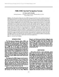
Figure 3.1: Orientation of axes The INS consists of 3-axis gyroscopes which give the system computer the roll, 7

pitch and yaw rates about the body axes as shown in figure 3.1 [23]. It also has 3-axis accelerometers which give the accelerations along the three body axes. There are two basic inertial mechanisms which are used to derive the Euler angles from the rate gyros, viz. stable platform and strap-down INS. We would be concerned with the strap-down INS where the gyros and accelerometers are ‘strapped-down’ to the aircraft body frame. The acceleration values from the accelerometers are then corrected for rotation of the earth and gravity to give the velocity and position of the aircraft.

3.1.1

Equations of Motion

The orientation of an aircraft with respect to a fixed inertial frame of axes is defined by three Euler angles. The aircraft is imagined to be oriented parallel to the fixed reference frame of axes. A series of rotations bring it to the orientation about axes OX, OY and OZ, as shown in figure 3.2 [23]: 1. clockwise rotation about the yaw axis, through the yaw (or heading) angle ψ , followed by 2. a clockwise rotation about the pitch axis, through the pitch angle θ, followed by 3. a clockwise rotation about the roll axis, through the bank angle φ. The relationship between the angular rates of roll, pitch and yaw, p, q, r (measured by the body mounted gyros), the Euler angles, ψ, θ, φ and their     ˙ φ 1 sin φ tan θ cos φ tan θ p      ˙     θ = 0 cos φ − sin φ   q     ˙ ψ 0 sin φ sec θ cos φ sec θ r

rates, is given below.     

(3.1)

By integration of the above equations we can derive the Euler angles using initial conditions of a known attitude at a given time. But, for pitch angles around ±90◦ , 8

Figure 3.2: Euler Angles the error becomes unbounded as tan θ tends to infinity. Quaternion algebra comes to the rescue here. We use four parameters, called the Euler parameters, that are related to the Euler angles as follows [24]. If e0 , e1 , e2 , e3 were the four parameters then in terms of angular rates, we have 1 e˙0 = − (e1 p + e2 q + e3 r) 2 1 e˙1 = (e0 p + e2 r − e3 q) 2 1 e˙2 = (e0 q + e3 p − e1 r) 2 1 e˙3 = (e0 r + e1 q − e2 p) 2

(3.2) (3.3) (3.4) (3.5)

with the parameters satisfying the following equation at all points of time. e0 2 + e 1 2 + e 2 2 + e 3 2 = 1

(3.6)

The above equations can be used to generate the time history of the four parameters e0 , e1 , e2 , and e3 . The initial values of the Euler angles are given which are used to 9

calculate the initial values of the four parameters using the following equations. θ φ ψ θ φ ψ cos cos + sin sin sin 2 2 2 2 2 2 ψ θ φ ψ θ φ e1 = cos cos sin − sin sin cos 2 2 2 2 2 2 ψ θ φ ψ θ φ e2 = cos sin cos + sin cos sin 2 2 2 2 2 2 θ φ ψ θ φ ψ e3 = − cos sin sin + sin cos cos 2 2 2 2 2 2 e0 = cos

(3.7) (3.8) (3.9) (3.10)

Once we have calculated the time history of the four parameters, we can calculate the Euler angles using the following equations. θ = sin−1 [−2(e1 e3 − e0 e2 )]  2  2 2 2 −1 e0 − e1 − e2 + e3 p φ = cos sign[2(e2 e3 + e0 e1 )] 1 − 4(e1 e3 − e0 e2 )2   2 2 2 2 −1 e0 + e1 − e2 − e3 p sign[2(e1 e2 + e0 e3 )] ψ = cos 1 − 4(e1 e3 − e0 e2 )2

(3.11) (3.12) (3.13)

We now have with us the attitude of the aircraft. To calculate the position we use the accelerations given by the accelerometers. The accelerations (ax , ay and az ) of the aircraft along the three body axes, as read by the accelerometers, are given by the equations 3.14 - 3.16. U , V , W and p, q, r are all available as states. If the acceleration due to gravity (g) model is supplied as ˙ can be calculated. a function of location around the earth, then U˙ , V˙ and W U˙ = aX + V r − W q + g sin θ

(3.14)

V˙ = aY − U r + W p − g cos θ sin φ

(3.15)

˙ = aZ + U q − V p − g cos θ cos φ W

(3.16)

The earth is rotating in space at a rate Ω (15◦ per hour) around an axis South to North as shown in figure 3.3. 

  Ω= 

Ω cos λ 0 −Ω sin λ 10

    

(3.17)

The motion of the vehicle at a constant height above the ground will induce an additional rotation given by 

  ω0 =  

µ˙ cos λ −λ˙ −µ˙ sin λ

    

(3.18)

The measured angular rates include Ω and ω 0 , we have the actual angular rates given

Figure 3.3: Local earth frame or Navigation frame by 







p p     h i     0  q  =  q  − DCM Ω + ω     r r

(3.19)

m

where DCM is the the direction cosine matrix or the transformation matrix, from the local earth or navigation frame to the body frame, given by equation 3.20, µ˙ is

11

the rate of change of longitude and λ˙ is the rate of change of latitude. .   cos θ cos ψ cos θ sin ψ − sin θ     DCM =  sin θ sin φ cos ψ − sin ψ cos φ sin ψ sin θ sin φ + cos ψ cos φ sin φ cos θ    sin θ cos φ cos ψ + sin ψ sin φ sin φ sin θ cos φ − cos ψ sin θ cos φ cos θ (3.20) ˙ are integrated to calculate the velocity components (U , V and W ), U˙ , V˙ and W which are then transformed using the direction cosine matrix (equation 3.20) to give velocity along North (VN ), velocity along East (VE ) and downward velocity (VD ) in the navigation frame or local earth frame, as shown in figure 3.3.       ˙ X V U    N     ˙       Y  =  VE  = DCMT  V        ˙ Z VD W

(3.21)

VN , VE and VD are then integrated to give distances moved along the navigation axes (X, Y, Z) on the surface of the earth. Let λ, µ and H denote the latitude, longitude and height of the aircraft at any instant, then rate of change of latitude [23, 25] is given by VN λ˙ = Re

(3.22)

and rate of change of longitude is given by µ˙ =

VE Re cos λ

(3.23)

where Re is the radius of the earth. The rate of change of altitude of the aircraft is given by H˙ = −VD

(3.24)

The position of the aircraft in terms of latitude, longitude and altitude can be thus calculated using equations 3.22, 3.23 and 3.24.

12

3.1.2

Errors in the INS

Most INS errors are attributed to the inertial sensors (instrument errors). These are the residual errors exhibited by the installed gyros and accelerometers following calibration of the INS. The dominant error sources are shown in table 3.1[6, 26]. Table 3.1: Sensor generated errors in the INS Alignment errors

roll, pitch and heading errors

Accelerometer bias or offset

a constant offset in the accelerometer output that changes randomly after each turn-on.

Accelerometer scale factor error

results in an acceleration error proportional to sensed acceleration.

Nonorthogonality of gyros

the axes of accelerometer and gyro

and accelerometers

uncertainty and misalignment.

Gyro drift or bias

a constant gyro output without angular

(due to temperature changes)

rate presence.

Gyro scale factor error

results in an angular rate error proportional to the sensed angular rate

Random noise

random noise in measurement

Errors in the accelerations and angular rates lead to steadily growing errors in position and velocity components of the aircraft, due to integration. These are called navigation errors and there are nine of them – three position errors, three velocity errors, two attitude errors and one heading error. If an unaided INS is used, these errors grow with time. It is for this reason that the INS is usually aided with either GPS, Doppler heading sensor or air-data dead reckoning systems. Gravity model can also cause some errors. The acceleration due to gravity varies from place to place along the earth and also with height. These errors have to be modelled accordingly. Inertial sensors for strapdown systems experience much higher rotation as compared to their gimballed counterparts. Rotation introduces error mechanisms that 13

require attitude rate-dependent error compensation.

3.2

Global Positioning System

3.2.1

Introduction

GPS uses a one-way ranging technique from the GPS satellites that are also broadcasting their estimated positions. Signals from four satellites are used with the user generated replica signal and the relative phase is measured. Using triangulation the location of the receiver is fixed. Four unknowns can be determined using the four satellites and appropriate geometry : latitude, longitude, altitude and a correction to the user’s clock. The GPS receiver coupled with the receiver computer returns elevation angle between the user and satellite, azimuth angle between the user and satellite, measured clockwise positive from the true north, geodetic latitude and longitude of the user. The GPS ranging signal is broadcast at two frequencies : a primary signal at 1575.42 MHz (L1 ) and a secondary broadcast at 1227.6 MHz (L2 ). Civilians use L1 frequency which has two modulations, viz. C/A or Clear Acquisition (or Coarse Acquistion) Code and P or Precise or Protected Code. C/A is unencrypted signal broadcast at a higher bandwidth and is available only on L1 . P code is more precise because it is broadcast at a higher bandwidth and is restricted for military use. The military operators can degrade the accuracy of the C/A code intentionally and this is known as Selective Availability. Ranging errors of the order of 100m can exist with Selective Availability. There are six major causes of ranging errors : satellite ephemeris, satellite clock, ionospheric group delay, tropospheric group delay, multipath and receiver measurement errors, including software. The primary role of GPS is to provide highly accurate position and velocity worldwide, based on range and range-rate measurements. GPS can be implemented in navigation as a fixing aid by being a part of an integrated navigation system, for 14

example INS/GPS.

3.2.2

Errors in GPS

Ephemeris errors occur when the GPS message does not transmit the correct satellite location and this affects the ranging accuracy. These tend to grow with time from the last update from the control station. Satellite clock errors affect both C/A and P code users and leads to an error of 1-2m over 12hr updates [27]. Measurement noise affects the position accuracy of GPS pseudorange absolute positioning by a few meters. The propagation of these errors into the position solution can be characterized by a quantity called Dilution of Precision (DOP) which expresses the geometry between the satellite and the receiver and is typically between 1 and 100. If the DOP is greater than 6, then the satellite geometry is not good. Ionospheric and tropospheric delays are introduced due to the atmosphere and this leads to a phase lag in calculation of the pseudorange.These can be corrected with a dual-frequency P-code receivers. Multipath errors are caused by reflected signals entering the front end of the receiver and masking the correlation peak. These effects tend to be more prominent due to the presence of reflective surfaces, where 15m or more in ranging error can be found in some cases.

3.3

Kalman Filtering

The Kalman Filter (KF) is a very effective stochastic estimator for a large number of problems, be it in computer graphics or in navigation. It is an optimal combination, in terms of minimization of variance, between the prediction of parameters from a previous time instant and external observations at a present time instant.

15

3.3.1

Discrete Kalman Filter

The KF addresses the general problem of trying to estimate the state x ∈