Majlesi Journal of Electrical Engineering
Vol. 4, No. 3, September 2010
Integration of Morphology and Graph-based Techniques for Fully Automatic Liver Segmentation Wan Nural Jawahir Hj Wan Yussof1, Hans Burkhardt2 1- Chair for Pattern Recognition and Image Processing, Albert-Ludwigs-Universität Freiburg, Freiburg, Germany Email:
[email protected] 2- Chair for Pattern Recognition and Image Processing, Albert-Ludwigs-Universität Freiburg, Freiburg, Germany Email:
[email protected]
Received: March 2010
Revised: May 2010
Accepted: July 2010
ABSTRACT: Here a fully 3D algorithm for automatic liver segmentation from CT volumetric datasets is presented. The algorithm starts by smoothing the original volume using anisotropic diffusion. The coarse liver region is obtained from the threshold process that is based on a priori knowledge. Then, several morphological operations is performed such as operating the liver to detach the unwanted region connected to the liver and finding the largest component using the connected component labeling (CCL) algorithm. At this stage, both 3D and 2D CCL is done subsequently. However, in 2D CCL, the adjacent slices are also affected from current slice changes. Finally, the boundary of the liver is refined using graph-cuts solver. Our algorithm does not require any user interaction or training datasets to be used. The algorithm has been evaluated on 10 CT scans of the liver and the results are encouraging to poor quality of images. KEYWORDS: Computed Tomography, 3D Liver segmentation Graph-cuts, Morphological Operations. 1. INTRODUCTION Recently, researchers of radiology and computer science struggle to solve liver segmentation from Computed Tomography (CT) image datasets either using semi-automatic [1], [3], [6], [9], [21] or fully automatic segmentation approaches [4], [7], [8], [14], [16], [18], [19]. Despite the great efforts put on this issue, the problem is still present due to several occurrences that make a liver the most difficult organ to be automatically segmented from an abdominal CT. We summarize the challenges reported in most publications as follows: • Adjacent organs (e.g., kidneys, spleen and stomach) might share similar gray levels. • The same organ may exhibit different gray level values. • The liver has a significant shape from one patient to another. • The acquired images have low contrast and blurred edges due to the partial volume effects. Based on our experience, using a 2D approach for volume liver segmentation was not efficient. The preliminary results offered in the Proceedings of International Conference on Soft Computing and Pattern Recognition 2009 [25] had a lack of accuracy. The algorithm was done in a slice-by-slice fashion. In this work, it was attempted to improve the quality of segmentation results using a 3D approach, with the
advantage that all three directions are treated simultaneously in comparison to the slice-by-slice manner. This paper is organized as follows: We report some related works in Section 2. In Section 3, we present our fully automatic liver segmentation algorithm using multi-morphological operations and graph-cuts techniques. Then, Section 4 reports our experimental results and finally we summarize our work in Section 5. 2. RELATED WORKS Many approaches to automatic liver segmentation have been presented in the literature, yet work in this area is ongoing. The approaches can be grouped into several categories but our reviews are limit on three most popular approaches: model-based, active contour and gray level based segmentation. 2.1. The Model-based Approach Most of the model-based approaches utilize the Statistical Shape Model (SSM) which was introduced by Cootes Et Al. [22]. SSM is a geometrical analysis of a set of shapes. Each shape in the training set is represented by a finite number of coordinate points, known as landmark points. Lamecker [6] built the SSM of liver from 20 manually segmented individual CT datasets. They proposed a geometric approach based on minimizing
59
Majlesi Journal of Electrical Engineering the distortion of the mapping given a few user-defined feature points where a user defines the feature points by decomposing the surface into patches. The patch boundaries were constructed by specifying only a few points on the surface and then computing the shortest path between them. The mean of the two 3D-shapes, were computed using a mere translation to align the gravity centers of the shapes and a rigid transformation computed by mean least squares (MLS). Principal Component Analysis (PCA) was used to analyze the variability over a set of training data to the set of corresponding liver surfaces. Heimann [19] trained the SSM on 35 training datasets to model the expected shape and appearance. The underlying SSM consists of 2,500 landmarks. Subsequently, a local search similar to the Active Shape method was used to initialize the main components of this approach which was a deformable mesh that strives for equilibrium between internal and external forces. The internal forces describe the deviation of the mesh from the underlying SSM, while the external forces model the fitness to the image data. They also employed a graph-based optimal surface detection during the calculation of the external forces.] 2.2. The Active Contour-based Approach The Active Contour developed by Kass Et Al. [10] also offers a means for image segmentation. The work was based on minimizing the energy, the sum of internal and external energy, associated to the current contour as shown in the following equation: snake
int
v
image
v
(1) v con where Eint represents the internal energy, Eimage gives rise to the image forces and Econ serves as external constrained forces. To yield a powerful computational object, Xu Et Al. [2] proposed a new type of external field called gradient vector flow (GVF) field and combined it with the usual internal forces. This type of active contour is called the GVF snake. The GVF snake has been used by Gui Et Al. [21] for semi-automatic liver segmentation. The first step of their algorithm was enhancing and denoising the images by histogram equalization and anisotropic diffusion filtering. Then several manually chosen points were connected using hemite-splines curve for the initial snake boundaries. Finally, fine segmentation was performed based on generalizing the GVF snake. Another work that used GVF for liver segmentation is reported in [16]. They used the canny edge detector to generate an edge map. A new maximum force angle map is introduced to evaluate the direction variability of the GVF forces. The segmentation was done in a slice-by-slice fashion.
60
Vol. 4, No. 3, September 2010 In the late nineties, the level set method has been widely used in various imaging domains including medical domains for liver segmentation [4], [7], [18]. The central idea supporting such an approach is to evolve the contour using a signed distance function, where its zero level corresponds to the actual contour. The algorithm proposed by Furukawa Et Al. [4] starts by a 2 maximum posterior (MAP) estimation using a probabilistic atlas of the liver. The atlas was constructed by applying the same normalization method to the label images obtained by manually segmenting the images in the training dataset. Then, the correction was done using level set based method on two terms, the geodesic term proposed by Caselles Et Al. [23] and another original term defined as the distance of a human body from the contour. The two-step seeded region growing (SRG) has been applied by Lee Et Al. [7] onto level-set speed images to define an approximate initial liver boundary. The first SRG efficiently divides a CT image into a set of discrete objects based on the gradient information and its connectivity. The second SRG detects the objects belonging to the liver based on a 2.5dimensional shape propagation, which models the segmented liver boundary of the slice directly above or below the current slice by evaluating the points to be narrow-banded, or by considering the local maximum of distance from the boundary. They utilized level-set speed images generally used for level-set propagation to detect the initial liver boundary. Finally, a rolling ball algorithm was applied to refine the liver boundary more accurately. 2.3. The Gray Level Based Approach Freiman Et Al. [9] proposed an adaptive hybrid segmentation algorithm using Bayesian classification on volume intensities. The process starts with a single user-defined pixel seed inside the liver. The mean and the variance of a rectangular neighborhood around this pixel is computed as the initial parameter values of the liver class. Then, a voxel classification with a smoothed MAP rule is applied to produce a segmentation label map. The identification of the liver region is done using an adaptive morphological adjustment to remove the disconnected regions outside the liver and to fill the holes inside the liver. Finally the liver volume is corrected by a level-set method. These three steps are repeatedly applied to the image until no further change occurs. Campedilli Et Al. [14] proposed another gray level based approach that involved three steps. The first step was preprocessing, which consists of finding the 'body box volume' where based on anatomical knowledge, a heart volume form is detected in successive slices. On the second stage, they defined a 3D box located below the heart volume that surely contains the liver tissue
Majlesi Jo ournal of Elecctrical Engineeering
Vol. 4, No. N 3, Septemb ber 2010
and calcullated the gray y level histograam within thee 3D box. The liver l gray leveel range was ddefined by finding the nearesst local minimu um at the left and the right side of the peaak. The estimaated liver grayy levels were then input in the t expansion n algorithm thhat segmented d the image by considering both the graay levels and the spatial rellationships am mong neighborring voxels. In n the last step, the t liver volum me was refineed by employin ng a 3D region n growing. M LOGY 3. THE METHODOL We prresent a hybrrid segmentattion method that integrates the morpholo ogical approacch with the graphcut techniique. Our segm mentation starrts by resizing g the image to one o half of itss original size in oder to red duce the compu utational time.. Then, we peerform a filter and threshold process to fin nd the coarse candidate reg gion. The multi-morphological operatorss and graph h-cut perform finer f correctio ons. The proccesses have been b done in a 3D 3 manner. otropic Diffussion for Noisee Filtering 3.1. Aniso To im mprove the reliability r off automatic liver l segmentattion algorithm ms, filtering techniques are required to t be used at the first stepp. The most basic b approach is to apply linear filters. Since CT imaages have im mportant and structured high frequeency componen nts like edges with fine dettails, linear fiilters such as th hose used in band-pass, hiigh-pass and lowl pass are not n suitable duee to the fact thhey might deg grade these imp portant structu ures. Thus, a nonlinear filter f should be used instead. In this case, each data poin nt is considered d separately an nd is either asssigned to noisse or a valid strructure. If thee point is definned as noise, it is simply rem moved and reeplaced by ann estimation based on the surrrounding data points. Parts oof the data that are not consid dered noise are a not modifi fied. Linear fiilters lack such a decision caapability and therefore, mo odify all data. One of the most fam mous nonlineaar filterings iss the anisotropic diffusion fiiltering. Pioneeered in 1990 0 by Perona an nd Malik [13]], anisotropic diffusion is also known ass the Perona and Malik equation. It was introduced d to MRI in 19 992 by Gerig Et. Al [5]. In [13] the smootthing method d is formulateed as a diffu usive process th hat is suppressed at boundarries using a paartial differentiaal equation (PD DE) of the form m: v,
div
v,
v,
(2)
where div v is a divergen nce operator annd ∇ is a grad dient operator. I in our case iss the 3D volum me of CT imag ge an v=(x,y,z) is i the coordin nate vector. A At each voxel,, the diffusion strength is controlled bby the so-caalled diffusion coefficient c((v,t) with t aas the processsing ordering parameter p useed to enumerate the iteraation steps. Thee diffusion co oefficient c(v,tt) depends on n the
mage gradient magnitude m ∇Ι. One popular form f is: im v, (3) v, exp Wh here the cond ductance paraameter , deteermines the con ntrast of edgees which has significant efffects on the sm moothing proceess. The succession of using g anisotropic difffusion for heelping in liverr segmentatio on has been rep ported in [24]. The use of a lookup l table for fo c(v,t) can draastically redu uce the computational timee. A detail maathematical fo ormulation of 3D anisotropic diffusion can n be referred d by [24]. Fig g. 1 shows a smoothing im mage resulted from fr anisotropiic diffusion.
(b) after filltering (a) before fiiltering Fig.1. The resu F ult from 3D anisotropic diffu usion using = after threee iterations. =35 2. The Estima ation of Liverr Gray Level 3.2 The distribu ution of the voxel intenssities holds meeaningful info ormation abou ut the 3D imaage content. Reelying on anato omical knowleedge in regard d to the liver volume, the in nformation contained in the image hisstogram can be b used to find d the initial liiver tissues. We use a priorii knowledge to t obtain the coarse liver reg gion. Our firstt assumption is i that, the disstribution of liv ver gray level is i always betw ween the valuees of 75 and 200. This range is used to fin nd the local maximum m of thee liver gray vaalues. We defiine this value as Ml . The coarse liver reg gion is obtain ned using two threshold values at the leeft and the rig ght side of th he Ml . The thrreshold values are given by: M M (4) M M We found th hat the values of α1 and α2 arre restricted by y the Ml valuee; such that th he greater the value v of Ml thee smaller the value of α1 and a α2 will bee. Then, the voxels which th heir intensity falls f between t1 and t2 are asssigned as part of the liver reegion. Otherw wise they are asssigned as the background b reg gion (0 valuess). 3.3 3. The Morph hological Opeerations Due to the fact f that some organs in a CT image shaare similar intensities, theree are several organs still rem maining afterr the thresho old process. We try to dissconnect smalll objects con nnected to a liver l region operations, usiing mathem matic morp phological speecifically open ning to break the connectio ons between
61
Majlesi Journal of Electrical Engineering the liver and the tissues which do not belong to it (e.g., kidneys). In mathematical morphology, opening is the dilation of a set I by a structuring element B as in the following equation: (5) Where and denote the erosion and dilation operator, respectively. The opening is done only in the z-direction to break the undesired tissues. Though the structuring element B takes care of the shape of the features while processing an image, it cannot equally treat the objects of the same shape but of the different size. Using multi-scale morphology as described in [17] such objects can expectantly be processed based on their shape as well as their size. This has been done using iteration number k=5 as the second attribute of the structuring element. Multi-scale filtering for opening is defined as: times
(6) … , Further on, a 3D connected component labeling (CCL) is used to extract the largest component. The positive aspect of using 3D CCL is its ability in preserving two liver regions that are not connected to each other in certain slices. However, the negative aspect is that it still keeps regions belonging to other tissues which are connected to adjacent slices of the liver. Therefore, 2D CCL is used after performing in three dimensions to complete the extraction of the largest component. To perform this operation, one has to specify the start slice and normally the best result can be produced if the start slice has the largest liver region. We approximate the start slice, cs as follows: (7) dim 0 ⁄2 dim 0 ⁄2 Where dim[0] is the size of volume in the zdimension and β∈[0,1] is determined based on the interior-slice distance. Aβ value should be larger if the distances are large. The 2D CCL in our scheme works from cs to dim[0] and from slice cs−1 to the first. We maintain the regions on the current slice, c that have region areas ≥250 due to our assumption that these regions might belong to the liver. The regions smaller than 250 are removed and the non-zero intensities in the c−1 and c+1 slices that have the same position (x,y) to these regions are also removed. In other words, we do not fully utilize the 2D process here but still take into account the adjacent slices. Then, in order to export the mask to the next slice, we perform one time dilation to the current mask. We do this step since it is assumed that the shape of the liver does not change dramatically in adjacent slices. In this way, the largest component in the next slice only can be searched within the mask. Those regions outside the mask are totally removed. ,
62
Vol. 4, No. 3, September 2010 3.4. Surface Reconstruction Using Graph Cut In this section, a graph-based approach is presented to refine the liver surface. In contrast to the active contour method for surface refinement, the graph-based method used in this work does not need to be done iteratively. It means the process can be done in only one single step. A graph G=(V,E) is a set of vertices V and a set of edges E. In the graph-cut scenario, there are two distinguished vertices in V called the source {s} and the sink {t} that will represent the labeling later. 3.5. The Proposed Formulation Given an initial contour obtained from the morphological segmentation as mentioned in the previous section, set of voxels is automatically defined which are considered to belong to the class object and background. The dilation and erosion operations are applied to the initial contour. Multi-scale erosion is performed to get the seed points of object O. For the background, B, the dilation process is only performed once and those voxels laying outside the region are considered as background. A binary variable xv is defined for each voxel v=(x,y,z) in O and B such that 1 v O (8) v 0 v B A discrete representation of the mean intensities in terms of the binary variables is adopted from [12] which is defined as follows: ∑ v v v O (9) ∑ v v O
∑
v B
v ∑ 1
v B
1
v
(10) v
The voxels are chosen from the start slice cs obtained by Eq. 7 as seed points for mean intensities of object and background. Since we are aiming at reconstructing the liver surface, only the voxels near the surface are considered. So, at this stage, we ignore the voxels which are certainly lie inside the liver volume or are part of the background. Thus, the subtraction between the dilated volume and the eroded volume is done. We denote the vertices as C. Let m1=(I(v)−c2)2 and m2=(I(v)−c1)2 such that v∈C. Then, for each vertex, we assign the weight to {s} and {t} as following: if (11) 0if or v 0 if (12) 0if or v 0 We represent the image as a 26-connectivity graph G=(V,E) which means each vertex v∈V in G, corresponding to a voxel p, has edges connecting to its
Majlesi Jo ournal of Elecctrical Engineeering 26 neighb boring verticees q denotes each neighbo oring voxel). For F each edg ge, we assignn the weightt as suggested by Boykov Ett Al. [26] as foollows: 1 ( (13) exp p . disp , 2 Where dissp(p,q) is the Euclidean E disttance between two voxels and can be evaluated e as thhe 'camera no oise'. The steps for the surfacce reconstructioon are graphiccally shown as in i Fig. 2.
(a)
(b)
(c)
(d)
(e)
Vol. 4, No. N 3, Septemb ber 2010 thee size 512x512 for each sliice. All CT im mages were enh hanced with contrast agen nts and were acquired in traansversal direcction. The pixeel spacing variied between 0.5 55 and 0.80 mm m and the in nter-slice disttance varied fro om 1 to 3mm with w no neighb boring slices ov verlapping. We used five different evaaluation metriics for the evaluation of ou ur segmentatio on results. Th hese metrics and their peculiaarities are giveen in [20]. Thee evaluation meetrics includee Volumetric Overlap Errror (VOE), Reelative Volu ume Differen nce (RVD),, Average Sy ymmetric Surfface Distance (SD), Root Mean M Square Sy ymmetric Surfface Distance (RMSD) and d Maximum Sy ymmetric Surfaace Distance (M MSD). The definitio on of these meetrics can be revised from Ap ppendix A. Taable 1 presentss the results fo or all the ten casses. The resullts have also been b visually presented p in Fig g. 3. For the majority m of thee ten cases, th he VOEs are lesss than 10%, while, w at the saame time, we achieved a the average of 2.99% % for the RVD D. The RMSD is below or clo ose to 2mm. Large MSD D are mostly caused by dev viations in th he region of the t vena cavaa and portal vein. Undersegm mentation occcurred when the lesions resside near the liiver edges (seee Fig. 3(c)). However, H the pro oposed segmeentation algoriithm proved to be robust forr different orieentations even n with poor qu uality of the im mages.
(a)
(b)
(c)
(d)
(f)
S reconsstruction usingg a graph-cut: (a) ( Fig. 2. Surface initiaal liver mask obtained o from morphology operations, (b) dilated liver mask, ((c) eroded liveer mask, (d) surface areas for graph-cut labeling, (e) after a applying graph-cut g on (d), white labells are voxels to o be removed from f (b) and (ff) final result aafter refining with w CCL. R AN ND DISCUSSIION 4. THE RESULTS To evaluaate the accuracy of the seggmentation ressults, we applied the proposeed method to 10 datasets1 with w
Fiig. 3. Segmenttation results from fr (a) slice 6 case 1, (b) sllice 6 case 2, (c) ( slice 2 casee 3 and (d) slicce 3 case 7. T segmentatiion results outtline is given in The n blue and referrence segmentaation is in red..
1
from http p://www.sliver0 07.org
63
Majlesi Journal of Electrical Engineering
Vol. 4, No. 3, September 2010
Table 1.Results of the segmentation metrics for all ten cases Datasets (slices)
Runtime
VOE [%]
RVD [%]
SD RMSD [mm] [mm]
MSD [mm]
6. ACKNOWLEDGMENT Here we would like to appreciate Dr. Raffi Enficiaud [15] for kindly sharing his C++ morphological library2 which significantly improved our segmentation speed.
1 (502)
5m48.533s
9.81
4.76
1.41
2.39
18.31
2 (358)
5m34.486s
11.02
3.59
1.51
2.85
22.47
REFERENCES
3 (244)
4m36.241s
12.23
2.55
2.48
4.93
37.46
4 (165)
3m08.225s
14.73
1.51
2.71
6.35
44.35
5 (91)
1m46.136s
9.85
-1.13
1.83
3.58
32.54
6 (258)
4m46.995s
8.63
2.22
1.33
2.65
24.94
7 (179)
3m21.479s
8.68
2.70
1.55
3.38
37.02
8 (97)
1m47.895s
9.81
8.15
1.63
2.62
21.01
9 (301)
5m37.645s
8.87
2.35
1.21
2.54
24.85
10 (73)
1m21.034s
9.46
3.16
1.63
3.66
30.57
10.31
2.99
1.73
3.49
29.35
[1] Beck A. and Aurich V.; “HepaTux – A Semiautomatic Liver Segmentation System”, 3D Segmentation in The Clinic: A Grand Challenge, pp. 225-233, (2007) [2] Xu C. and Prince J.L.; “Snakes, Shapes and Gradient Vector Flow”, IEEE Transactions on Image Processing, Vol. 7, pp. 359-369, (1998) [3] Chen E.L., Chung P.C. and Tsai H.M. and Chang C.I.;“An Automatic Diagnostic System for CT Liver Image Classification”, IEEE Transactions on Biomedical Engineering, Vol. 45, No. 6, pp. 783-794, (1998) [4] Furukawa D., Shimizu A. and Kobatake H.; “Automatic Liver Segmentation Method based on Maximum A Posterior Probability Estimation and Level Set Method”, 3D Segmentation in The Clinic: A Grand Challenge, pp. 117-124, (2007) [5] Gerig G., Kübler O., Kikinis R. and Jolesz F.A.; “Nonlinear Anisotropic Filtering of MRI Data”, Medical Imaging, IEEE Transactions, Vol. 11, No. 2, pp. 221-232, (1992) [6] Lamecker H., Lange T. and Seebass M.; “A Statistical Shape Model for the Liver”, In Proc. Medical Image Computing and Computer Assisted Intervention, Vol. 2489, pp. 422-427, (2002) [7] Lee J., Kim N., Lee H., Seo J.B., Won H.J., Shin Y.M., Shin Y.G. and Kim S.H.; “Efficient Liver Segmentation Using a Level-Set Method with Optimal Detection of the Initial Liver Boundary from Level-set Speed Images”, Computer Methods and Programs in Biomedicine, Vol. 88, pp. 26-38, 2007. [8] Ma L. and Yang L., “Liver Segmentation Based on Expectation Maximization and Morphological Filters in CT Images”, IEEE, pp. 690-693, (2007) [9] Freiman M., Eliassaf O., Taieb Y., Joskowicz L., Azraq Y. and Sosna J.; “An Iterative Bayesian Approach for Nearly Automatic Liver Segmentation: Algorithm and Validation”, International Journal CARS, Vol. 3, pp. 439-446, (2008) [10] Kass M., Witkin A. and Terzopoulos D.; “Snakes: Active Contour Models”, International Journal of Computer Vision, pp. 321-331, (1988) [11] Aspert N., Cruz D.S. and Ebrahimi T.; “MESH: Measuring Errors Between Surfaces Using The Hausdorff Distance”, In Proc. of the IEEE International Conference in Multimedia and Expo, Vol. 1, pp. 705-708, (2002) [12] El-Zehiry N. and Elmaghraby A.; “An Active Surface for Volumetric Image Segmentation”, In Proc. of Biomedical Imaging: From Nano to Macro (ISBI 2009), pp. 1358-1361. (2009) [13] Perona P. and Malik J.; “Scale-space and Edge
Average
5. CONCLUSION Automatically segmenting the liver is not easy and multiple techniques are required to perform this task. Most of the liver segmentation algorithms that had already been published in the literature have their own advantages. Nevertheless, those algorithms are not applicable in all situations. For example, using the SSM method does not promise good results if the number of training datasets is very small. Similarly, although many applications in computer vision used active contour technique and some actually achieved good results, but for the application where segmentation serves as a preprocessing step such as where it is used for content-based image retrieval (CBIR), it requires a lot of time to execute. In concern to the above matter, the algorithm proposed in this paper takes into account, the computational time and the number of datasets we have. We propose a hybrid approach using morphological-based and graph-based techniques. Morphology opening and connected component labeling were used in this work concentrating on finding liver regions and removing other regions from the volume. While graph-cuts technique focuses on refining the surface of the liver volume. Our segmentation process runs without user intervention. The maximum computational time is less than 6 minutes on an Intel(R) Core(TM) Duo CPU with 3GHz and 7.7GB RAM. Another advantage of our approach is that it does not demand for a training phase which is often troublesome. Our algorithm works natively in 3D and shows an improvement in the term of its accuracy in comparison to the previous work that was performed in a slice-by-slice manner.
2
http://raffi.enficiaud.free.fr
64
Majlesi Journal of Electrical Engineering
[14]
[15]
[16]
[17]
[18]
[19]
[20]
[21]
[22]
[23] [24]
[25]
Detection Using Anisotropic Diffusion”, IEEE Trans. on Pattern Analysis and Machine Intelligence, Vol. 12, pp. 629-639, (1990) Campadelli P., Casiraghi E. and Esposito A.; “Liver Segmentation from Computed Tomography Scans: A Survey and a New Algorithm”, Artificial Intelligence in Medicine, Vol. 45, pp. 185-196, (2009) Enficiaud R., “Algorithmes Multidimensionnels et Multispectraux en Morphologie Mathématique: Approche par Méta-programmation”, Centre de Morphologie Mathématique - École des Mines de Paris, (2007) Huang S., Wang B. and Huang X.; “Using GVF Snake to Segment Liver from CT Images”, Proceedings of the 3rd IEEE-EMBS International Summer School and Symposium on Medical Devices and Biosensors, pp. 145-148, (2006) Lim S.J., Jeong Y.Y. and Ho Y.S.; “Automatic Liver Segmentation for Volume Measurement in CT Images”, Journal of Visual Communication and Image Representation, Vol. 17:4, pp. 860-875, (2006) Pan S., Dawant B.M.; “Automatic 3D segmentation of the Liver from Abdominal CT Images: A Level Set Approach”, Proc. of SPIE Medical Imaging 2001: Image Processing, Vol. 4322, pp. 128-138, (2001) Heimann T., Meinzer H.P. and Wolf I., “A Statistical Deformable Model for the Segmentation of Liver CT Volumes”, 3D Segmentation in The Clinic: A Grand Challenge, pp. 161-166, (2007) Heimann T., B. Van Ginneken, Styner M.A. and Arzhaeva Y., Aurich V., Bauer C., Becker A., Beichel R., Bekes G., Bello F., Binnig G., Bischof H., Bornik A., Cashman P.M.M., Chi Y., Córdova A., Dawant B.M., Fidrich M., Furst J.D., Furukawa D., Grenacher L., Hornegger J., Kainmüller D., Kitney R.I., Kobatake H., Lamecker H., Lange T., Lee J., Lennon B., Li R., Li S., Meinzer H.P., Németh G., Raicu D.S., Rau A.M., Van Rikxoort E.M., Rousson M., Ruskó L., Saddi K.A., Schmidt G., Seghers D., Shimizu A., Slagmolen P., Sorantin E., Soza G., Susomboon R., Waite J.M., Wimmer A. and Wolf I., “Comparison and Evaluation of Methods for Liver Segmentation From CT Datasets”, IEEE Transactions on Medical Imaging, Vol. 28, pp. 1251-1265, (2009) Gui T., Huang L.L. and Shimizu A.; “Liver Segmentation for CT Images Using an Improved GGVF-Snake”, SICE Annual Conference 2007, pp. 676-681, (2007) Cootes T.F., Taylor C.J., Cooper D.H. and Graham J.; “Active Shape Models - Their Training and Application”, Computer Vision and Image Understanding, Vol. 61, pp. 38-59, (1995) Caselles V., Kimmel R. and Sapiro G., “Geodesic Active Contours”, International Journal of Computer Vision, Vol. 22, pp. 66-79, (1995) Yussof W.N.J.W. and Burkhardt H.; “3D Anisotropic Diffusion for Liver Segmentation”, Proceedings of World Academy of Science, Engineering and Technology, Vol. 57, pp. 108-112, (2009) Yussof W.N.J.W. and Burkhardt H.; “3D Liver Segmentation using Hybrid Segmentation Techniques”, Proceedings of the International
Vol. 4, No. 3, September 2010 Conference of Soft Computing and Pattern Recognition, pp. 404-408, (2009) [26] Boykov Y. and Lea G.F.; “Graph Cuts and Efficient N-D Image Segmentation”, International Journal of Computer Vision, Vol. 70, Issue 2, pp. 109–131, (November 2006)
APPENDIX A. The Evaluation Metrics In the following evaluation metrics, VM and VA are the set of voxels from manual segmentation and the set of voxels from automatic segmentation, respectively. SM denotes the set of surface voxels of VM and SA denotes the set of surface voxels of VA. Before we describe five error measures, let us first define the shortest distance of an arbitrary voxel v to the set of surface voxel S as follows: v,S min v (A.1) Where ||.|| denotes the Euclidean distance. If we replace the voxel v in the Equation A.1 with vm where vm SM and S with SA then the shortest distance d(vm,SA) is obtained for the voxel in the set SM to the set SA. And we get d(va ,SM) for va SA, vice versa. Following comes the five error measures used to evaluate our segmentation results. • Volumetric Overlap Error: This metric measures the percentage of mismatching voxels between the automatic and manual segmentation. The percentage of volumetric overlap error between VM and VA is defined as: V V VOE 100 1 (A.2) V V Where for a perfect segmentation the value of Equation A.2 is 0% otherwise it takes the value 100% when there is no overlap at all between VM and VA. • Relative Volume Difference: The relative volume difference between VM and VA is given in percent and is defined as: V V (A.3) RVD 100 V Where for a perfect segmentation the value of Equation A.3 is 0%. • Average Symmetric Surface Distance: The average symmetric surface distance is defined as the average of all stored distances. For clarity, the stored distances are defined as follow: D S ,S
v ,S v
S
v
S
D S ,S
v ,S
•
(A.4)
•
(A.5)
Then, the average symmetric surface distance is given by:
65
Majlesi Journal of Electrical Engineering SD
S
* D S ,S
S
Vol. 4, No. 3, September 2010 (A.6)
D S ,S
This value is 0 for a perfect segmentation. • Root Mean Square Symmetric Surface Distance: In contrast to the previous metric, the Euclidean distance between surface voxels are squared before storing them. D S ,S
v ,S v
S
v
S
D S ,S
(A.7)
v ,S
(A.8)
After averaging the squared values, the root is extracted and the symmetric RMS surface distance is given, which is 0 for a perfect segmentation. 1
RMSD
S
S
* D S ,S
(A.9)
D S ,S
• Maximum Symmetric Surface Distance: This metric is also known as the Hausdorff distance [11]. The determination of this metric is similar to the previous two metrics, but only the maximum of all voxel distances is taken instead of the average. The maximum surface distance between SM and SA, denoted by dm(SM,SA) and dm(SA,SM) are given by: max sm, S m S ,S • (A.10) sm S
m
and S ,S
max
sa S
sa, S
,
•
(A.11)
Respectively. Then, the symmetrical Hausdorff distance is defined as follows: MSD
max
m
S ,S ,
m
S ,S
(A.12)
When the distance is 0, it means a perfect segmentation has been achieved.
66