Integration of Multiple Temporal Qualitative Probabilistic Networks in ...

Integration of Multiple Temporal Qualitative Probabilistic Networks in Time Series Environments Yali Lv 1, 2 1

School of Computer Science and Technology, Tianjin University, Tianjin, 300072, China

Shizhong Liao 1, * 2

School of Information management, Shanxi University of Finance & Economics, Taiyuan, 030006, China

* Corresponding author’s Email: [email protected]

Abstract: The integration of uncertain information from different time sources is a crucial issue in various applications. In this paper, we propose an integration method of multiple Temporal Qualitative Probabilistic Networks (TQPNs) in time series environments. First, we present the method for learning TQPN from time series data. The TQPN’s structure is constructed using Dynamic Bayesian Networks learning based on Markov Chain Monte Carlo. Furthermore, the corresponding qualitative influences are obtained by the conditional probabilities. Secondly, based on rough set theory, we integrate multiple TQPNs into a single QPN that preserves as much information as possible. Specifically, we take the rough-set-based dependency degree as the strength of qualitative influence, and then make the rules to solve the ambiguities reduction and cycles deletion problems which arise from the integration of different TQPNs. Finally, we verify the feasibility of the integration method by the simulation experiments. Keywords: Qualitative Probabilistic Networks; Temporal Qualitative Probabilistic Networks; Integration; Time Series Environments; Markov Chain Monte Carlo; Rough Sets

1. Introduction Temporal Qualitative Probabilistic Network (TQPN) is an important knowledge representing method in Artificial Intelligence. Sometimes, the knowledge-based systems need not only to be learned from the time series data, but also to be integrated into a single network for representing the consensus probabilistic knowledge in the whole time series environments. There are many kinds of networks which can be used to represent the probabilistic knowledge, such as Bayesian Networks (BNs) [1], Dynamic Bayesian Networks (DBNs) [2,3], Qualitative Probabilistic Networks (QPNs) [4] and Temporal Qualitative Probabilistic Networks (TQPNs) [5]. BN has been established as a framework for representing uncertain probabilistic knowledge. The

general methods for learning BN from data have been studied [6,7], including the corresponding analysis and evaluation. Li and Liu [8] have integrated multiple dependency structures of BNs based on the generalized relation model and constructed a large BN that preserves as much information as possible. Sagrado et al. [9] have obtained the consensus BN model by combining two graphs and applying the union and intersection of their independencies. However, the qualitative and temporal nature in time series environments can not be represented by these methods. In order to describe the temporal information in practice, DBN, as the extension of BN in the discrete time and discrete state of stochastic processes, is used to represent the system states by time slices. The strictly numeric representations of BN and DBN are inappropriately for many applications. In many cases, we only need to know

International Journal of Intelligent Engineering and Systems, Vol.3, No.2,2010

9

the qualitative probabilistic knowledge. Considering the trade-off between efficiency and precision to some extent, QPN was proposed by Wellman [4], as the qualitative abstraction of a BN. However, it can not represent the temporal nature of probabilistic knowledge. Based on these ideas, Liu and Yue [5] have proposed TQPN and implemented the qualitative and temporal knowledge representation. They construct TQPN's structure by considering the relationships between variables existing not only in each time slice, but also in adjacent time slices. However, in some cases, since the relationships always follow the time flow, only the relationships existing in adjacent time slices need to be considered. Yue et al. [10] have also investigated the qualitative representation and integration of probabilistic causalities in multiple time slices, they only considered to delete the cycles between two variables. In fact, the cycle formed by more than two variables may exist in the integration process. Therefore, it is a worthy effort to learn TQPNs from data, and then to integrate multiple TQPNs into a single QPN. In this paper, we first present the method for learning each TQPN from each group time series data. Secondly, we integrate the multiple TQPNs into a QPN that preserves as much information as possible in the whole time series environment. The rest of this paper is organized as follows. In the following section, we introduce the preliminaries on QPN and TQPN. Section 3 proposes the method for learning TQPN from time series data and integrating multiple TQPNs based on rough set theory. Section 4 shows the experimental results and the corresponding analysis. Finally, Section 5 concludes this paper.

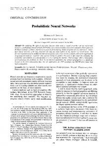
QPN abstracted from a BN is shown in Figure 1. A qualitative influence between variables expresses how the values of one variables A influence the probabilities of the values of the other variable B , denoted by S δ ( A, B) , δ ∈ {+, −,0,?} . p(x1 ) = 0.5 X1

X3

+ p(x4 |x2 , x3 ) = 0.99 p(x4 |x2 , x¯3 ) = 0.90 p(x4 |¯x2 , x3 ) = 0.90 X4 p(x4 |¯x2 , x¯3 ) = 0.00 (a) BN

+ X4

(b) QPN

Figure 1. An example of QPN abstracted from BN.

Definition 1 [4] A positively influences B , denoted by S + ( A, B) , iff for all x ∈ π ( B ) \ { A} such

P (b | ax) − P (b | ax) ≥ 0, where π ( B ) \ { A} is the parents set of B other than A . The definition expresses the fact that observing a high value for A makes the higher value for B more likely, regardless of any other direct influences on B . A negative influence, denoted by S − , and a zero influence, denoted by S 0 , are defined analogously, just substituting ≤ and = for ≥ respectively. If the influence of A on B is positive for one combination of x and negative for another combination, the influence is called ambiguous influence, denoted by S ? . The set of qualitative influences exhibits the properties of symmetry, transitivity and composition: z The property of symmetry guarantees that, if a network includes the influence S δ ( A, B) , it

z

2.1 Qualitative Probabilistic Networks A Qualitative probabilistic network (QPN) encodes variables by the directed acyclic graph (DAG) like a BN, and summarizes the probabilistic relationships between variables by qualitative influences on the directed edges [4]. For abbreviation, all variables are assumed to be binary and ordered, writing a for A = True (or A = 1 ) and a for A = False (or A = 0 ), in which a > a (or 1 > 0 ). A simple example of

+

p(x |x ) = 0.8 X3 p(x3 |¯x1 ) = 0.2 =⇒ X2 3 1

p(x2 |x1 ) = 0.1 p(x2 |¯x1 ) = 0.5 X2

2. Preliminaries In this section, we will review several basic concepts of QPN and TQPN.

X1 −

z

also includes S δ ( B, A) with the same sign. That is, S δ ( A, B) ⇔ S δ ( B, A). The property of transitivity asserts that qualitative influences along an active trail without nodes with two incoming arcs combine into an indirect influence whose sign is determined by ⊗ − operator from Table 1. This is, S δ1 ( A, B) ⊗ S δ 2 ( B, C ) ⇒ S δ1 ⊗δ 2 ( A, C ). The property of composition asserts that multiple qualitative influences between two variables along parallel active trails combine into a composite influence whose


10

sign is determined by ⊕ − operator from Table 1. That is, S δ1 ( A, C ) ⊕ S δ 2 ( A, C ) ⇒ S δ1 ⊕δ 2 ( A, C ). Table 1. The ⊗ − and ⊕ − operators ⊗

+ - 0 ?

⊕

+ - 0 ?

+

+ - 0 ?

+

+ ? + ?

-

- + 0 ?

-

? - - ?

0

0 0 0 0

0

+ - 0 ?

?

? ? 0 ?

?

? ? ? ?

2.2 Temporal Qualitative Probabilistic Networks Definition 2 [5] A temporal qualitative probabilistic network (TQPN) is a directed acyclic graph Gt ,t +1 = (V , Q ) , describing the causal relationships of

variables in time Tt , Tt +1 and Tt →( t +1) , denoted by Gt ,

Gt +1 and Gt →t +1 respectively, where z V = Vt U Vt +1 is the set of variables in Tt and Tt +1 ; z

Q = {+, −,0,?} is

the

set

of DBN. Let X

{

= X

[t ] 1

,X

[t ] 2

,..., X n

[t ]

} denote

the

random variables in X at time t ∈ {1, 2,...} . Figure 2 displays a simple example of TQPN. There are six variables in the adjacent time slices t and t + 1 . X1t

X1t+1

−

−

X2t

−

− +

+

+

X2t+1

+ X3t +

3.1 Learning TQPN from Time Series Data

The main goal of learning the structure of TQPN or DBN is to find a model M that best fits the data D . The scoring metric is the posterior probability P ( M | D ) . According to the Bayes rule, the posterior probability can be written as P( D | M ) P( M ) P(M | D) = , (1) P( D) where P ( D ) is a constant that does not depend on M . Therefore, taking logarithm, a scoring function for a model M can be built as S ( M ) = log P ( D | M ) + log P ( M ). (2) Given the scoring criteria, a common approach is to find the highest scoring network. However, the appropriateness of searching for only the highest scoring network may be questionable, at least in a small sample dataset. So the full posterior distribution over network models can be considered in this case.

of qualitative

influences on the directed edges in Gt ,t +1 . Analogously, TQPN is the qualitative abstraction [t ]

framework of multiple TQPNs is shown in Figure 3.

X3t+1

Figure 2. A simple example of TQPN between two adjacent time slices.

3. Integration of multiple TQPNs In this section, we first learn each TQPN from the corresponding time series data of each group, and then integrate the multiple TQPNs into a single QPN, namely the integrated QPN (IQPN) which can preserve as much information as possible in the whole time series environment. The integration

3.1.1 Markov Chain Monte Carlo Method

The idea of Markov Chain Monte Carlo (MCMC) method [2,3] is to construct a Markov chain in which a new model M * is generated only in terms of the previous one M . It will produce a chain of models that converge to the target distribution eventually. Metropolis-Hastings (MH) algorithm is one of the most important MCMC methods. For each run, the algorithm will sample a new candidate model from the jumping distribution J ( M * | M ) , given the candidate model M * , the acceptance probability can be computed as P ( M * | D) J ( M | M *) Ac = min{ 1, × }. (3) P(M | D) J ( M * | M ) 3.1.2 Learning the Structure of TQPN

Given n groups of time series data D1 , D2 , ..., Dn , we find each model M = (G , Q ) from the corresponding data of each group, where G denotes the structure of TQPN and Q is the qualitative influences between variables. Since the relationship between variables always follows the time flow, it’s unnecessary to consider the qualitative influences in the same time slice Gt and Gt +1 , so the directed arcs are only permitted between the adjacent time slices Gt →t +1 as Figure 4(a).


11

Figure 4(b) expresses no unrolling TQPN followed

Learning each TQPN

Integrating multiple TQPNs

{

by time point, so it is a directed cyclic graph.

time series data1

time series data2

...

time series datan

TQPN1

TQPN2

...

TQPNn

{

The Integrated QPN

Figure 3. The integration framework of multiple TQPNs in the whole time series environment.

hyperparameter of the Dirichlet distribution, r α ij = ∑ k =1α ijk . Γ(⋅) is Gamma function.

X1t X1t+1

X1

− X2t

− +

+

−

=⇒

X2t+1

+

X2

X3t

X3

+

X3t+1

+

3.1.3 Learning Qualitative Signs

−

+

(a)

(b) Q

Figure 4. TQPN without considering the relationships between variables in the same time slices. (a) The corresponding TQPN by unrolling the right network followed by time point. (b) A simple TQPN, where X 2 and X 3 form a multi-node loop, and X 3 has a self-loop.

In this paper, we use the approach to learn DBN based on MCMC method [2,3] to construct the structure of TQPN. Similarly, we also assume to be first order Markov and discrete model. Here we obtain the last sample model in the chain of models, and regard it as the convergence of the target distribution. According to the global and local parameter independence assumptions, the scoring function in Equation (2) can be decomposed as n

S ( M ) = ∑ S ( M ii ),

(4)

i =1

where n is the number of variables. The BDe criterion [3] can be obtained as S BDe ( M i ) = log P(Gi ) + q

Γ(α i j )

∏ Γ(α j =1

ij

r

∏

Γ(α i jk + N i jk ) Γ(α i jk )

+ N i j ) k =1

Since the precise numbers are not relevant for the ordering task, the reasoning in terms of frequencies is generally perceived as less demanding than the reasoning in terms of probabilities [11]. We can use the frequencies format for representing the conditional probabilities. Thus, by statistical computations on the given sample data, and Definition 1, we can easily obtain the probability orderings, and then conclude the corresponding qualitative relationships. 3.1.4 Learning Algorithm

The algorithm for learning TQPN from time series data is described as Algorithm 1. Algorithm 1 Learning TQPN from Time Series Data Input: D ( time series data); N (number of sampling) Output: A TQPN= (G , Q) 1: Set initial model M 0 ; 2: for i = 0 to N do

3:

sample a new model M *

4:

compute the acceptance probability Ac ;

5:

sample u U [0,1] ;

6:

if Ac > u then M i +1 ← M * ;

7:

, (5)

J (M * | M i ) ;

8: 9:

else M i +1 ← M i ;

10: end if

where r , q is the total number of discrete state of X i and its parents node Pai , respectively. N ijk is the

11:

sufficient statistics, X i = xk with Pai = pa j occurs

13: Select the last sampling model M as G ;

over all time slices, N ij = ∑ k =1 N ijk . α ijk is the r

M ← M i +1 ;

12: end for 14: Compute the qualitative signs Q in G ;


12

R β X = { x ∈ U | P ( X / [ x ]R ) ≥ β } ,

15: return A TQPN= (G, Q) .

Where J ( M * | M ) is based on the neighborhood concept of a given network M , named N ( M ) that can be obtained from M with a single edge removal or addition [12], i.e., for all M * ∈ N ( M ) , J ( M * | M ) = 1 / N ( M ) . For TQPN, we have N ( M ) = n 2 , regardless of M . For TQPN, in this paper, edges are only allowed between the adjacent time slices, so there is no acyclic and equivalence problems. In addition, the restriction on the number of fan-ins and the cost of computation for TQPN can be considerably alleviated. 3.2 Integrating Multiple TQPNs Based on Rough Set Theory

The integration of multiple TQPNs includes the structure integration and qualitative sign integration. Let {TQPN1, TQPN2, …, TQPNn } be n TQPNs. In this subsection, we will show how to integrate n TQPNs into a single QPN, namely a integrated QPN (IQPN) which can preserve the information as much as possible in the whole time series environment. 3.2.1 Rough Set Theory

The rough set theory has been proposed by Pawlak [13,14] and widely applied to model imprecise or incomplete knowledge. According to Pawlak’s rough set theory, the zero dependency degree can be associated with the qualitative influence whose strength should not be zero actually [15], so Yue et al. [15] adopted the probabilistic rough set theory to obtain dependency degree as the strength between the associated variables. Let U be the universe of discourse and R be an equivalence relation over U . The equivalence relation R partitions the set U into disjoint subsets. This partition of the universe is called a quotient set induced by R , denoted by U / R . It represents a very special type of similarity between elements of the universe. According to [13-15], we redescribe the following three definitions. Definition 3 Let X be a set of objects in U and R be an equivalence relation over U . Let β (0.5 < β ≤ 1) be a given threshold value. Let P be the probabilistic measure defined on U . The probabilistic lower approximation of X with respect to R is defined as

where P ( X / [ x]R ) =

| X I [ x ]R | , | ⋅ | denotes the [ x ]R

amount of elements, and [ x]R represents the set of objects in U that are equivalent to x with respect to R . Definition 4 Given two families of equivalence relations A and B , and the threshold value β (0.5 < β ≤ 1) , POS Aβ ( B ) = U X ∈U / B Aβ X is called

the positive domain of B with respect to A . Actually, POS Aβ ( B) is the set of objects in U / A that are also in U / B . Definition 5 Let γ Aβ ( B ) = | POSA β ( B) | | U | . γ is

called the degree that B depends on A not less than probability β , written A ⇒ γβ B(0 ≤ γ ≤ 1) . The amount of elements in | POS Aβ ( B) | and that in U are denoted by | POS Aβ ( B) | and | U | . 3.2.2 The Qualitative Signs Integration

We observe that combining multiple non-ambiguous qualitative signs along parallel active trails in the same QPN, can yield an ambiguous result, i.e., such an ambiguity arises when parallel influences with opposite signs are combined with ⊕ − operator in Table 1. To reduce the ambiguities, Yue et al. [15] introduced the rough-set-based dependency degree as the strength of qualitative influence. We use the following Example 1 to illustrate the rough-set-based dependency degree. Example 1 Suppose ( X 1 , X 2 ) be a directed edge in the QPN and each variable value be binary. The given sample data is shown in Table 2. Let us consider the dependency degree between variable X 1 and X 2 . We set β = 0.6 , since | X 2 = 0 I X1 = 0 | | X 2 = 0 I X 1 = 1| = 0.5 < β , = 0.29 < β , | X1 = 0 | | X 1 = 1| | X 2 = 1 I X1 = 0 | | X 2 = 1 I X 1 = 1| = 0.5 < β , = 0.71 > β , | X1 = 0 | | X 1 = 1|

thus X 1 X = { X 1 = 1} = {Ns = 1,3,4,6,8,9,15} . According to Definition 4 and Definition 5, we have γ X ( X 2 ) = γ ( X1, X 2 ) =

|POS X1 ( X 2 ) |

1

| Ns |

= 0.47.

Similarly, γ X ( X1 ) = 2


|POS X 2 ( X 1 ) | | Ns |

= 0.4.

13

Table 2. The given sample data. V denotes the variables X 1 and X 2 , Ns denotes the sample number. V \ Ns X1 X2

1-5

6-10

11-15

10110 11111

10110 00101

00001 01001

X1 − X2

X1

?

−

+

? X3

X2

X1

?

+

?

(a) TQPN1

(b) TQPN2

−

+ X3

X2

?

X3

+ +

(c) TQPN3

Figure 5. The parallel active trails and the corresponding qualitative signs in three TQPNs.

Similarly, we can also introduce it to reduce ambiguities in integrating the qualitative signs of multiple TQPNs, and regard the same nodes and the directed edge in two graphs as the parallel active trail, i.e., edge ( X 1 , X 2 ) in Figure 5 is the parallel active trail when we integrate TQPN1 and TQPN2. Obviously, combining multiple non-ambiguous qualitative signs with ⊕ − operator, along parallel active trails in the different TQPNs, can also yield an ambiguous result, i.e., combining two signs of ( X 1 , X 2 ) in TQPN1 and TQPN2 in Figure 5, the ambiguity, "− ⊕+ = ?" , arises. In addition, combining the ambiguous qualitative signs, or, combining the signs of edge ( X 3 , X 1 ) , ( X 2 , X 3 ) , ( X 3 , X 2 ) in Figure 5(a) and 5(b) respectively, can yield the ambiguous results too. The results are "?⊕ − = ?" , "?⊕ ? = ?" ,"+ ⊕ ? = ?" . In this paper, we still use Definition 6 [15] to reduce these ambiguities. Definition 6 (Parallel Active Trails Combination) S δ [γ ] ( X 1 , X 2 ) = S δ1 [γ 1 ] ( X 1 , X 2 ) U S δ 2 [γ 2 ] ( X 1 , X 2 ) (0 < γ 1 , γ 2 ≤ 1) , where δ and γ are defined as follows: z If δ1 = δ 2 , then δ = δ1 = δ 2 and γ = γ 1 + γ 2 − γ 1 ⋅ γ 2 . z If δ1 ≠ δ 2 and γ 1 > γ 2 , then δ = δ1 and γ = γ 1 − γ 2 + γ 1 ⋅ γ 2 . z If δ1 ≠ δ 2 and γ 1 < γ 2 , then δ = δ 2 and γ = γ 2 − γ 1 + γ 1 ⋅ γ 2 . z If δ1 ≠ δ 2 , and γ 1 = γ 2 , then δ = δ1 ⊕ δ 2 and γ = γ 1 = γ 2 .

3.2.3 The Structure Integration

We know, a QPN is a directed acyclic graph and each TQPN without unrolling followed by time point is directed cyclic graph. The topological integration is based on the union of graph structure [9,10]. In this paper, we combine the structure of multiple TQPNs based on the graph union, too, which will generate more cycles. Therefore, we need to deal with the cycles problem in the process of the structure integration. The more edges the IQPN has, the more information it preserves. According to the integration goal, we make the following rules for deleting the cycles in the graph union of multiple TQPNs (UTQPN). Rule 1: If there exists the cycles in the UTQPN and the only one edge can be deleted to make the UTQPN acyclic, we directly delete the edge. For example, while integrating TQPN1 and TQPN2 in Figure 5 into a QPN, we must delete edge ( X 2 , X 3 ) rather than ( X 3 , X 2 ) , because the UTQPN has no cycle in this case and the IQPN preserves the information as much as possible. Rule 2: If the only one edge doesn't exist, let N ( X 1 , X 2 ) be the occurrence number of edge ( X 1 , X 2 ) in all TQPNs, We will find the cycle with the biggest N and then delete the edge with the smallest N in the cycle. For example, while integrating TQPN1 and TQPN3 in Figure 5, since N ( X 2 , X 3 ) = N ( X 3 , X 2 ) = 2, N ( X 1 , X 2 ) = N ( X 2 , X 1 ) = 1, we would find the cycle that formed by ( X 2 , X 3 ) and ( X 3 , X 2 ) , and then delete ( X 2 , X 3 ) or (X3, X2 ) . Rule 3: If each N in the cycle is equal, we delete the edge with the smallest dependence degree γ . For example, if γ X 2 ( X 3 ) > γ X 3 ( X 2 ) β

β

in the example of Rule 2, we delete edge ( X 3 , X 2 ) , or delete ( X 2 , X 3 ) . Rule 4: If there exists the self loop in the UTQPN, we can regard it as a particular case of Rule 2 and 3. For example, X 3 has a self loop in Figure 5(b), we can regard N ( X 3 , X 3 ) or γ X 3 ( X 3 ) as the β

smallest one in the cycle, so we can delete it. That is, we can directly delete the self loop in each TQPN, which does not change the final integration result.


14

3.2.4 The Integration Algorithm

4. Experiments

The integration method of multiple TQPNs basically consists of three steps. 1. Do preprocessing and delete the self loop in each TQPN by Rule 4; 2. Add all edges and the qualitative signs into the UTQPN, and record the occurrence number N of each edge in all TQPNs, and integrate qualitative signs according to Definition 6. 3. Delete the cycles in the UTQPN according to Rule 1, 2 and 3, and conclude a single QPN, or IQPN. Thus, the integration algorithm of multiple TQPNs is summarized as Algorithm 2.

4.1 Experiment Setup

Algorithm 2 Multiple TQPNs Integration Algorithm Input: TQPN1, TQPN2, …, TQPNn ; all γ Output: A integrated QPN, or IQPN

1: Delete all self loop in each TQPN; 2: m ← nodes number;

All the methods have been implemented in Matlab by making use of Markov chain Monte Carlo software [12] and Bayes net toolbox [16]. 4.2 Time Series Data

In the experiment, we will integrate two TQPNs into a single QPNa assuming all data to be binary and complete. Two groups time series data are generated by a predefined DBN and simulated using Matlab, and shown in Table 3 and 4. There are 8 variables ( A[t ] , B[t ] , C [t ] , D[t ] , A[t +1] , B[t +1] , C [ t +1] , D[ t +1] ) and 100 time points, respectively. Table 3. The first group of time series data. X denotes variables, T denotes time points from 1 to 100.

X \T A[ t ]

3: for k = 1 to n do

…

4: for i = 1 to m do 5:

for j = 1 to m do

D[ t ] A[t +1]

… 6:

Add edge Eij k and sign δ ij k to UTQPN;

7:

if Eij k = EijU then

8:

NE U ← NE U + 1 ; ij

9:

D[t +1]

1

2

1

0

1 0 0

3

4

5

6 … 98 99 100

1 … 0 1 0 0 … 0 0

1

0

1 1

1 0

1

0

1 … … 1 … 1 … … 1 …

0

1

0

0 1

0 1

0 0

1

0

0

Table 4. The second group time series data. X denotes variables, T denotes time points from 101 to 200.

ij

SU δ [γ ] = SU δ [γ ] U S k δ [γ ] ;

X \T A[t ]

10:

end if

…

11:

end for

D[ t ] A[t +1]

12: end for 13: end for

… [ t +1]

D

101 102 0

103

104

0

0

1 1

0 1

0

1

0 …

1 0

0 1

0

1

…

… 198 199 200 … … … … ... …

1

1

0

0 1

0 0

1 1

1

1

0

14:while there exists the cycles in the UTQPN do 15: Delete the only one edge that makes the UTQPN acyclic; 16: if the edge doesn't exist then 17:

Find the cycle with the biggest N ;

18:

Delete the edge with the smallest N ;

19:

if each N in the cycle is equal then

Delete the edge with the smallest γ ; 21:

end if

22: end if 23: end while 24:IQPN ← UTQPN; 25:return IQPN.

4.3 Experimental Results and Analysis

We first use Algorithm 1 to learn TQPN1 between two adjacent time slices from the first group data, and learn TQPN2 from the second group data, respectively. The number of sampling is 2000 and the max fan-in is 3. The structure graphs of two TQPNs with unrolling the network followed by time point are concluded as Figure 6 by Algorithm 1. According to the known data, we can learn the conditional probability orderings. Thus we obtain two corresponding TQPNs without unrolling Figure 6 followed by time point, which are shown in Figure 7.


15

At

At At+1

At+1

Bt

Bt B

t+1

give the node order [B,C,D,A] according to Figure 8(a). The max fan-in is set as 3. The final QPN that abstracted from the corresponding BN is shown in Figure 8(b). B

B t+1

B +

?

Ct

C t+1

−

Dt+1

Dt+1

(b) TQPN2 structure

Figure 6. The two structures of TQPN with unrolling the network followed by time point. + B

+ +

?

+ −

D

+ +

?

C

C +

D −

? +

?

A

A

(b) TQPN2

(a) TQPN1

Figure 7. The two corresponding TQPNs without unrolling Figure 6 followed by time point.

Further, we set β = 0.6 and compute the dependency degree of two variables on the directed edge in two TQPNs, and obtain the rough-set-based influence strength that is shown in Table 5. We integrate the two TQPNs into a single QPN by Algorithm 2, and then conclude the integrated QPN as Figure 8(a). Table 5. The qualitative influence strength in two TQPNs. γ denotes the influence strength on the corresponding edge. γ TQPN1 TQPN2

( B, C ) 0.54 ( A, D) 0.2

(C , A) 0.44 ( B, C ) 0.49

+ −

D

Dt

B

C

+

C t+1

(a) TQPN1 structure

?

C

Ct

Dt

+

(C , B ) (C , D) ( D, A) ( B, B) ( D, D) 0.56 0.62 0.58 1 1 ( B, D) (C , B ) (C , D) ( D, A) ( D, B ) 0.51 0.43 0.43 0.9 0.89

In order to verify the feasibility of our methods, we use the general BN learning method, like K2 Algorithm, to learn QPN from the whole dataset. We

−

D ?

A

A

(a) The integrated QPN

(b) The learned QPN by a BN method

Figure 8. (a) The integrated QPN in the whole time series environments. (b) The learned QPN by a general BN method.

Comparing two QPNs in Figure 8(a) and Figure 8(b), we conclude that the two results are consistent with each other. The qualitative sign on edge ( D, A) is '− ' in Figure 8(a), and that in Figure 8(b) is '?' , which is not contradictory, because we use the rough-set-based influence strength to reduce the ambiguity in the integrated QPN. In addition, given two TQPNs and small sample data with 30 time points, we can also obtain the same integration result by Algorithm 2. Therefore, to some extent, our methods outperform K2 as follows. z Our methods show the temporal nature in time series environments. z K2 Algorithm needs to elicit the topological ordering, but our methods don't. z Given multiple TQPNs, we can directly integrate multiple TQPNs into a single QPN with the small dataset. For K2 Algorithm, a relatively large dataset is needed to learn a QPN.

5

Conclusions and Further Research

In this paper, in order to represent qualitative and temporal probabilistic knowledge coming from different time sources, we propose an integration method of multiple TQPNs and construct a single QPN that preserves as much information as possible. However, there are many important aspects deserving future attention, like how to integrate multiple QPNs that come from different information sources, and how to evaluate the integration result, it includes the integrated structure evaluation and the integrated qualitative signs evaluation.


16

Acknowledgments This work is supported in part by Natural Science Foundation of China under Grant No. 60678049 and Natural Science Foundation of Tianjin under Grant No. 07JCYBJC14600.

References [1] J. Pearl, Probabilistic Reasoning In Intelligent Systems: Networks of Plausible Inference. San Mateo, CA: Morgan Kaufmann Publishers, 1988. [2] H. Lahdesmaki and I. Shmulevich, “Learning the structure of dynamic Bayesian networks from time series and steady state measurements”, Machine Learning, Vol.71, pp.185-217, 2008. [3] H. Wu and X. Liu, “Dynamic Bayesian networks modeling for inferring genetic regulatory networks by search strategy: Comparison between greedy hill climbing and MCMC methods”, in: Proc. of World Academy of Science, Engineering and Technology, vol.34, pp. 224-234, 2008. [4] M. P. Wellman, “Fundamental concepts of qualitative probabilistic networks,” Artificial Intelligence, Vol.44, pp. 257-303, 1990. [5] W. Y. Liu, K. Yue, S. X. Liu, and Y. B. Sun, “Qualitative-probabilistic-network-based modeling of temporal causalities and its application to feedback loop identification ”, Information Sciences, Vol.178, No.7, pp.1803-1824, 2008. [6] G. F. Cooper and E. Herskovits, “A Bayesian method for the induction of probabilistic networks from data”, Machine Learning, Vol. 9, pp.309-347, 1992. [7] J. Cheng, R. Greiner, J. Kelly, D. Bell and W. Liu, “Learning Bayesian networks from data: An information-theory based approach”, Artificial Intelligence, Vol.137, pp.43-90, 2002. [8] W. H. Li, W. Y. Liu, and Z. Y. Zhang, “Integrating dependency structure of multi Bayesian networks”, in: Proc. of the 3rd International Conf. on Machine Learning and Cybernetics, pp.26-29, 2004. [9] J.del Sagrado and S. Moral, “Qualitative combination of Bayesian networks”, International Journal of Intelligent Systems, Vol.18, pp.237-249, 2003. [10] K. Yue, M. H. Gao, G. Han, and W. Y. Liu, “Qualitative representation and fusion of probabilistic causalities in time-series environments”, Journal of Yunnan University, Vol.31, No.5, pp 455-462, 2009. [11] G. Gigerenzer and U. Hoffrage, “How to improve Bayesian reasoning without instruction: Frequency formats”, Psychological Review, Vol.102, pp.684-704, 1995. [12] D. Husmeier, “Sensitivity and specificity of inferring genetic regulatory interactions from microarray experiments with dynamic Bayesian networks”, Bioinformatics, Vol.19, No.17, pp. 2271-2282, 2003. [13] Z.Pawlak, “Rough sets”, International Journal of Computer and Information Sciences, Vol.11, pp.

341-356, 1982. [14] Z. Pawlak, Rough Sets: Theoretical Aspects of Reasoning about Data, Kluwer Academic Publishers, 1991. [15] K. Yue, Y. Yao, J. Li, and W. Y. Liu, “Qualitative probabilistic networks with reduced ambiguities”, Applied Intelligence, online: DOI 10.1007/s10489-008-0156-5, 2008. [16] K. P. Murphy, “The Bayes net toolbox for Matlab”, Computing Science and Statistics, Vol.33, pp.1-20, 2001, software is available on-line at http://bnt.sourceforge.net/.


17