INTEGRATION OF PHOTOGRAMMETRIC AND LIDAR DATA IN A MULTIPRIMITIVE TRIANGULATION PROCEDURE A.F. Habib, K.I. Bang, M. Aldelgawy University of Calgary, Department of Geomatics Engineering, Canada
[email protected],
[email protected],
[email protected] S. W. Shin, K. O. Kim Spatial Information Research Team, Telematics & USN Research Division Electronics and Telecommunications Research Institute, South Korea
[email protected],
[email protected]
ABSTRACT Photogrammetry is the art and science of deriving accurate metric and descriptive information from analog and digital images. Photogrammetric reconstruction produces surfaces that are rich in semantic information, which can be clearly recognized in the captured imagery. The inherent redundancy associated with photogrammetric restitution results in highly accurate surfaces. Nevertheless, the amount of effort and time required by the photogrammetric reconstruction procedure is a major disadvantage. In LIDAR mapping, however, spatial coordinates of object space points are directly acquired, enabling quick turnaround of mapping products. Still, the positional nature of LIDAR points makes it difficult to derive semantic surface information such as discontinuities and types of observed structures. Additionally, no inherent redundancy is available in the reconstructed surfaces that may be utilized to enhance the accuracy of the final product. The complementary characteristics of photogrammetry and LIDAR, if exploited, can lead to a more complete surface description. The synergic advantages of both systems can be fully realized only after precise calibration of both systems and successful registration of the photogrammetric and LIDAR data relative to a common reference frame. Generally, a registration methodology has to deal with three issues: registration primitives, transformation function, and similarity measure. In this paper, two methodologies are introduced for the co-registration of LIDAR and photogrammetric datasets. One track of methodologies uses straight-lines while the other uses planar patches as the registration primitives. The mathematical model and similarity measures corresponding to both types of primitives are introduced. The presented approaches can be divided into two categories. The first category includes new constraints that can be added to current bundle adjustment procedures. On the other hand, the second category utilizes existing point-based bundle adjustment procedures after manipulating the variance-covariance matrices of the linear and areal primitives. The proposed methodologies are tested and proved efficient in a multi-sensor triangulation environment. For the feasibility test, IKONOS stereo-pair and medium-format aerial image block are integrated with LIDAR data in a single bundle adjustment procedure while implementing linear and areal features.
INTRODUCTION A diverse range of spatial data acquisition systems is now available onboard satellite, aerial, and terrestrial mapping platforms. The diversity starts with analog and digital frame cameras and continues to include linear array scanners. In the past few years, imaging sensors witnessed vast development as a result of an enormous advancement in the digital technology. For example, the increasing sensor size and storage capacity of digital frame cameras lead to their application in traditional and new mapping functions. However, due to technical limitations, current digital frame cameras are not capable of providing geometric resolution and ground coverage similar to those associated with analog frame cameras. To alleviate such a limitation, push-broom scanners (line cameras) have been developed and used onboard satellite and aerial platforms. However, rigorous modeling of the imaging process of push-broom scanners is far more complicated than the modeling of frame sensors (Poli, 2004; Toutin, 2004-a; Toutin, 2004-b). For example, in the absence of the georeferencing parameters, the narrow Angular Field of View (AFOV) associated with current push-broom scanners are causing instability in the triangulation procedure due to strong correlation between the components of the Exterior Orientation Parameters (EOP). Therefore, there has been a tremendous body of research that dealt with the derivation of alternative models for line cameras to circumvent such instability (Tao et al, 2004; Habib et al, 2004; Fraser and Hanley, 2003). In addition to line cameras, the low cost of medium-format digital frame cameras is leading to their frequent adoption by the mapping community. Apart from imaging systems, LIDAR scanning is rapidly taking its place in the ASPRS 2007 Annual Conference Tampa, Florida May 7-11, 2007
mapping industry as a fast and cost-effective 3D data acquisition technology. The increased accuracy and affordability of GPS/INS systems are the main reasons behind their expanding role in orienting LIDAR sensors. Considering the characteristics of acquired spatial data from imaging and LIDAR systems, one can argue that their integration will be beneficial for accurate and complete description of the object space. It is evident that the disadvantages of one system can be compensated for by the advantages of the other system (Baltsavias, 1999; Satale and Kulkarni, 2003). However, the synergic characteristics of both systems can be fully utilized only after ensuring that both datasets are georeferenced relative to the same reference frame (Habib and Schenk, 1999). Traditionally, photogrammetric geo-referencing is either indirectly established with the help of Ground Control Points (GCP) or directly defined using GPS/INS units on board the imaging platform (Cramer et al, 2000). On the other hand, LIDAR geo-referencing is directly established through the GPS/INS components of a LIDAR system. In this regard, this paper presents alternative methodologies for utilizing LIDAR features as a source of control for photogrammetric geo-referencing. These methodologies have two main advantages. First, they will ensure the co-alignment of the LIDAR and photogrammetric data to a common reference frame as defined by the GPS/INS unit of the LIDAR system. Moreover, LIDAR features will eliminate the need for ground control points to establish the geo-referencing parameters of the photogrammetric data. The possibility of utilizing LIDAR data as a source of control for photogrammetric geo-referencing hinges on the ability to identify common features in both datasets. Therefore, the first objective of the developed methodologies is concerned with the selection of appropriate primitives. Afterwards, the mathematical models, which can be utilized in the triangulation procedure, for relating LIDAR and photogrammetric primitives will be introduced. The paper will start by offering a brief discussion of the appropriate primitive for relating the LIDAR and photogrammetric data as well as the respective mathematical models for their incorporation in the triangulation procedure. The feasibility and the performance of the developed multi-primitive and multi-sensor triangulation will be outlined through the experimental results section using real data. Finally, the paper will conclude with final remarks and recommendations for future research.
APPROPRIATE PRIMITIVES A triangulation process relies on the identification of common primitives for relating the involved datasets to the reference frame defined by the control information. Traditionally, photogrammetric triangulation has been based on point primitives. Considering photogrammetric and LIDAR data, relating the laser footprint to the corresponding point in the imagery is almost impossible. Therefore, point primitives are not appropriate for the task at hand. Linear and areal features are other potential primitives that can be more suitable for relating LIDAR and photogrammetric data. Linear features can be directly identified in the imagery while conjugate LIDAR lines can be extracted through planar patch segmentation and intersection. Alternatively, LIDAR lines can be directly identified in the intensity images produced by most of today’s LIDAR systems. It should be noted that extracted linear features from planar patch segmentation and intersection are more accurate than the extracted features from intensity images. The lower quality of extracted features from the intensity images is caused by the utilized interpolation process for converting the irregular LIDAR footprints to a raster grid. Other than linear features, areal primitives in photogrammetric datasets can be defined using their boundaries, which can be identified in the imagery. Such primitives include, for example, roof tops, lakes, and other homogeneous regions. In LIDAR datasets, areal regions can be derived through planar patch segmentation techniques. Another issue that is related to the primitives selection is their representation in both photogrammetric and LIDAR data. In this regard, image space lines can be represented by a sequence of image points along the feature. This is an appealing representation since it can handle image space linear features in the presence of distortions as they will cause deviations from straightness in the image space. Furthermore, such a representation will allow for the inclusion of linear features in scenes captured by line cameras since perturbations in the flight trajectory would lead to deviations from straightness in image space linear features corresponding to object space straight lines (Habib et al., 2002). It should be noted that the selected intermediate points along corresponding line segments in overlapping scenes need not be conjugate. As for the LIDAR data, object lines can be represented by their end points. The points defining the LIDAR line need not be visible in the imagery. For areal primitives, photogrammetric planar patches can be represented by three points (e.g., corner points) along their boundaries. These points should be identified in all overlapping imagery. Similar to the linear features, this representation is valid for scenes captured by frame and line cameras. On the other hand, LIDAR patches can be represented by the footprints defining that patch. These points can be directly derived from planar patch segmentation techniques. Having settled the primitive selection and representation issues, the next section will focus on explaining the proposed mathematical models for relating the photogrammetric and LIDAR primitives within the triangulation procedure.
ASPRS 2007 Annual Conference Tampa, Florida May 7-11, 2007
LINEAR FEATURE CONSTRAINTS This section introduces the proposed alternative procedures for the incorporation of control lines, which are derived from LIDAR data, in a bundle adjustment procedure. The first approach outlines a new constraint that can be added to current bundle adjustment procedures. The second approach utilizes existing bundle adjustment procedures for the incorporation of linear features after manipulating the variance-covariance matrices associated with the points representing image and/or object space linear features.
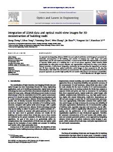
Coplanarity-based Incorporation of Linear Features This section will focus on deriving the mathematical constraint for relating LIDAR and photogrammetric lines, which are represented by the end points in the object space and a sequence of intermediate points in the image space, respectively. From this perspective, the photogrammetric datasets will be aligned to the LIDAR reference frame through direct incorporation of LIDAR lines as the source of control. The photogrammetric and LIDAR measurements along corresponding linear features can be related to each other through the coplanarity constraint in Equation 4. This constraint indicates that the vector from the perspective centre to any intermediate image point along the image line is contained within the plane defined by the perspective centre of that image and the two points defining the LIDAR line. In other words, for a given intermediate point, k˝, the points {(X1, Y1, Z1), (X2, Y2, Z2), (X”0, Y”0, Z”0), and (xk”, yk”, 0)} are coplanar, Figure 1. r r r (V1 × V2 ) • V3 = 0 (1) Where r V1 is the vector connecting the perspective centre to the first end point along the LIDAR line, r V2 is the vector connecting the perspective centre to the second end point along the LIDAR line, and r V3 is the vector connecting the perspective centre to an intermediate point along the corresponding image line. It should be noted that the above constraint can be introduced for all the intermediate points along the image space linear feature. Moreover, the coplanarity constraint is valid for both frame and line cameras. For scenes captured by line cameras, the involved EOP (Exterior Orientation Parameters) should correspond to the image associated with the intermediate point under consideration. For frame cameras with known IOP (Interior Orientation Parameters), a maximum of two independent constraints can be defined for a given image. However, for self-calibration procedures, additional constraints will help in the recovery of the IOP since the distortion pattern will change from one intermediate point to the next along the image space linear feature. On the other hand, the coplanarity constraint would help in better recovery of the EOP associated with line cameras. Such a contribution is attributed to the fact that the system’s trajectory will affect the shape of the linear feature in the image space. ( X O′ , YO′ , Z O′ )
( X O′′ , YO′′, Z O′′ )
(Ω ′′, Φ ′′, Κ ′′) (Ω′, Φ′, Κ′)
⎡ X 2 − X O′′ ⎤ → V 2 = ⎢⎢ Y2 − YO′′ ⎥⎥ ⎣⎢ Z 2 − Z O′′ ⎦⎥
⎡ x k ′′ − x p − d is t or t ion s x ⎤ → V 3 = R (Ω ′′, Φ ′′, Κ ′′)⎢⎢ y k ′′ − y p − d is t or t ion s y ⎥⎥ ⎢⎣ ⎥⎦ −c
⎡ X 1 − X O′′ ⎤ → V 1 = ⎢⎢ Y1 − YO′′ ⎥⎥ ⎢⎣ Z1 − Z O′′ ⎥⎦
Figure 1. Perspective transformation between image and LIDAR straight lines and the coplanarity constraint for intermediate points along the line.
ASPRS 2007 Annual Conference Tampa, Florida May 7-11, 2007
Collinearity-based Incorporation of Linear Features in Existing Bundle Adjustment Procedures In contrast to the above approach, existing bundle adjustment procedures, which are based on the collinearity equations, can be used to incorporate linear features after the modification of the variance-covariance matrices associated with the line measurements either in the object or image space. Before getting into the implementation details of this approach, we will start by outlining the representation methodology of the linear features. Similar to the previous approach, object space lines will be represented by two points. On the other hand, image space linear features will be represented by two points, which are not conjugate to those defining the line in the object space, Figure 2. However, the image and object space points will be assigned the same identification code. The fact that these points are not conjugate will be tolerated by manipulating their variance-covariance matrices either in the image or object space. In other words, the variancecovariance matrix of a given point will be expanded along the linear feature to allow for its movement along the line direction. For example, Equations 2-6 explain the methodology of expanding the error ellipse associated with an end point in the image space, refer to Figure 3. First, we need to define the xy- and uv-coordinate systems. The xy-coordinate system is the image coordinate system, Figure 3-a. On the other hand, the uv-coordinate system is a coordinate system with the uaxis aligned along the image line, Figure 3-b. The relationship between these coordinate systems is defined by a rotation matrix, Equation 2. This rotation matrix is defined by the image line orientation. Using the law of error propagation, the variance of the end point in the uv-coordinate system can be derived from the variance-covariance matrix in the xycoordinate system, Equation 3, according to Equation 4. To allow for the point movement along the line, the variance along the u-axis is replaced by a large value (simply by multiplying the respective variance by a constant m), Equation 5. Finally, the modified variance-covariance matrix in the xy-image coordinate system is calculated by the utilization of the inverse rotation matrix as in Equation 6, Figure 3-c. The same procedure can be used to expand the variance-covariance matrix of the end points for the object lines.
∑ ∑
uv
⎡u ⎤ ⎡ x⎤ ⎢v ⎥ = R ⎢ y⎥ ⎣ ⎦ ⎣ ⎦
(2)
⎡σ 2 =⎢ x ⎢⎣ 0
(3)
xy
=R
xy
⎡m × σ u2 σ uv ⎤ =⎢ ⎥ σ v2 ⎥⎦ ⎣⎢ σ uv
∑
'
uv
∑
∑
0⎤ ⎥ σ y2 ⎥⎦ ⎡ σ 2 σ uv ⎤ RT = ⎢ u 2⎥ ⎣⎢σ uv σ v ⎥⎦
' xy
= RT
∑
' uv
R
Figure 2. Representation of image and object lines for the collinearity-based incorporation of linear features in bundle adjustment. ASPRS 2007 Annual Conference Tampa, Florida May 7-11, 2007
(4)
(5) (6)
The decision whether to expand the variance-covariance matrix in the image or object space depends on the procedure under consideration (e.g., single photo resection, bundle adjustment of an image block using control lines, bundle adjustment of an image block using tie lines). 1. Single Photo Resection using control lines (Figure 4-a): In this approach, the image line will be represented by two end points with their variance-covariance matrices defined by the expected accuracy of image coordinate measurement accuracy. On the other hand, the variance-covariance matrices of the end points of the control line are expended to compensate for the fact that the image and object points are not conjugate. It should be noted that this approach can be still used for single photo resection of a scene captured by line camera. 2. Single Photo Resection using control lines (Figure 4-b): In this approach, the object line will be represented by its end points, whose variance-covariance matrices are defined by the expected accuracy of the utilized procedure for defining these points. On the other hand, the variance-covariance matrices of the image line are expanded along its direction. One should note this approach is not appropriate for scenes captured by line camera, since the image-line orientation cannot be rigorously defined at a given point due to perturbations in the flight trajectory. However, the line orientation along the scene can be used as an approximation. 3. Bundle adjustment of an image block using control lines (Figure 4-c): In this approach, the object line will be represented by its end points with their variance-covariance matrices defined by the utilized procedure for providing the control lines. On the other hand, the variance-covariance matrices of the image lines are expanded to compensate for the fact that the end points of the image lines are not conjugate to those defining the object line. It should be noted that this approach is not appropriate for scenes captured by line cameras since the image line orientation cannot be rigorously defined. 4. Bundle adjustment of an image block using control lines (Figure 4-d): In this case, the image lines in overlapping images will be represented by non-conjugate end points whose variance-covariance matrices are defined by the expected accuracy of the image coordinate measurement accuracy. To compensate for the fact that these points are not conjugate to each other, the selected end points will be assigned different identification codes. On the other hand, the object line will be defined by a list of points whose variance-covariance matrices are expanded. The number of the object points depends on the number of the selected points in the image space. It should be noted that this approach can be used for scenes captured by frame or line cameras since it does not require the expansion of the variance-covariance matrix in the image space. 5. Bundle adjustment of an image block using tie lines (Figure 4-e): In this approach, all variance-covariance matrices associated with the end points of the image lines will be expanded except for two points. These points will be used to define the object line. Since this approach requires an expansion of the error ellipse in the image space, it is not appropriate for scenes captured by line cameras since the image line orientation cannot be rigorously defined due to perturbation in the flight trajectory. Figure 4-f illustrates the conceptual basis of the derivation of the object point through the proposed variance-covariance manipulation. The image point with an error ellipse, which is established by the image coordinate measurement accuracy, together with the corresponding perspective center defines an infinite light ray. On the other hand, the image point with the expanded error ellipse together with the corresponding perspective center defines a plane. The intersection of the light ray and the plane leads to the estimation of the ground coordinates of the point in question.
Figure 3. Expanding the error ellipse associated with an end point of an image line.
ASPRS 2007 Annual Conference Tampa, Florida May 7-11, 2007
y q1 y x
p1
x
q2
p2
Q1 P1 y
Z W U
v
Y Control line P2
P2
V
σU
q1
Q2
X
x
σu
u Control line
(b)
(a)
y2
p'1
p1
y1 x1
y1 x1
x2
p'2
Error ellipse of q1
q1
p1
Q1
y2 q2
x2
p2
p2
P1
P1
Control line
Observed point Adjusted point Q2
Error range Error range
Control line
Error range
(c)
y1 x1
P2
P2
(d)
p'1
p1
y2
Residual of an image point measurement p'2
x2
p2 P1
y1 x1
p'1
p1
y2 x2
P1 Tie line
(f) P2
(e)
Figure 4. Variance expansion options of line end points for their incorporation in collinearity-based bundle adjustment procedures.
AREAL FEATURE CONSTRAINTS This section introduces the proposed alternative procedures for the incorporation of control patches, which are derived from LIDAR data, in a bundle adjustment procedure. The first approach outlines a new constraint that can be added to current bundle adjustment procedures. The second approach utilizes existing bundle adjustment procedures for the incorporation of areal features after manipulating the variance-covariance matrices associated with the points representing object space areal features. ASPRS 2007 Annual Conference Tampa, Florida May 7-11, 2007
Coplanarity -based Incorporation of Areal Features This section will focus on deriving the mathematical constraint for relating LIDAR and photogrammetric patches, which are represented by a set of points in the object space and three points in the image space, respectively. As an example, let us consider a surface patch that is represented by two sets of points, namely the photogrammetric set SPH= {A, B, C} and the LIDAR set SL= {(XP, YP, ZP), P=1 to n}, Figure 5-a. Since the LIDAR points are randomly distributed, no point-topoint correspondence can be assumed between the datasets. For the photogrammetric points, the image and object space coordinates will be related to each other through the collinearity equations. On the other hand, LIDAR points belonging to a certain planar-surface patch should coincide with the photogrammetric patch representing the same object space surface, Figure 5-a. The coplanarity of the LIDAR and photogrammetric points can be mathematically expressed through Equation 7. a c
a
c
y1
y1
a
x1
x2
x1
b
b
y2
c
y2
b
b
a
c
x2
C
C
A Z
A Z
Y
Y
X
B
X
B
(a)
(b)
Figure 5. Coplanarity-based (a) and collinearity-based (b) incorporation of LIDAR patches in photogrammetric triangulation. X P YP X A YA V= X B YB X C YC
ZP ZA ZB ZC
1 X P − X A YP − YA 1 = X B − X A YB − YA 1 X C − X A YC − YA 1
ZP − Z A ZB − Z A = 0 ZC − Z A
(7)
The above constraint is used as the mathematical model for incorporating LIDAR points into the photogrammetric triangulation. In physical terms, this constraint means that the normal distance between any LIDAR point and the corresponding photogrammetric surface should be zero, or the volume of the tetrahedron comprised of the four points is equal to zero. This constraint is applied for all LIDAR points comprising this surface patch.
Collinearity-based Incorporation of Areal Features in Existing Bundle Adjustment Procedures In this approach, existing bundle adjustment procedures, which are based on the collinearity equations, can be used for incorporating control areal features after the manipulation of the variance-covariance matrices defining the control patch. Similar to the previous approach, the planar patch in the image space will be defined by a set of vertices that can be identified in overlapping imagery. On the other hand, the control patch will be defined by an equivalent set of object points (i.e., identical number of vertices defining the image and object patch). However, the object points need not be conjugate to those identified in the image space, Figure 5-b. To compensate for the fact that these sets of points are not conjugate, the variance-covariance matrices of the object points are expanded along the plane direction (Equations 8-12, Figures 6). In these equations, the XYZ-coordinate system defines the ground reference frame. On the other hand, the UVW-coordinate system is defined by the orientation of the control patch in the object space. Specifically, the UV-axes are defined to be parallel to the plane through the patch (i.e., the w-axis is aligned along the normal to the patch). The expansion of the error ellipsoid along the plan is facilitated by multiplying the variances along the U and V directions by large numbers (e.g., mU and mV in Equation 11). It should be noted that this approach is suitable for scenes captured by frame and line cameras. The conceptual basis of the collinearity-based incorporation of areal patches in existing bundle adjustment procedures is illustrated in Figure 6.
ASPRS 2007 Annual Conference Tampa, Florida May 7-11, 2007
⎡X ⎤ ⎡U ⎤ ⎢V ⎥ = R ⎢ Y ⎥ ⎢ ⎥ ⎢ ⎥ ⎣⎢ Z ⎦⎥ ⎣⎢W ⎦⎥
∑ ∑
UVW
∑
'
UVW
=R
⎡σ X2 ⎢ =⎢ 0 ⎢ 0 ⎣
XYZ
∑
XYZ
⎡mU × σ U2 ⎢ = ⎢ σ VU ⎢ σ ⎣ WU
∑
' XYZ
0
σ Y2 0
(8) 0 ⎤ ⎥ 0 ⎥ σ Z2 ⎥⎦
⎡ σ U2 ⎢ R T = ⎢σ VU ⎢σ ⎣ WU
σ UV σ V2 σ WV
(9)
σ UW ⎤ ⎥ σ VW ⎥ σ W2 ⎥⎦
(10)
σ UV σ UW ⎤ ⎥ mV × σ V2 σ VW ⎥ σ WV σ W2 ⎥⎦
(11)
∑
(12)
= RT
'
UVW
R
Figure 6. Conceptual basis of the collinearity-based incorporation of control areal patches in existing bundle adjustment procedures.
EXPERIMENTAL RESULTS To validate the feasibility and applicability of the above methodologies, multi-sensory datasets were solicited and analyzed. The conducted experiments involved four types of sensors: namely, a digital frame camera equipped with a GPS receiver, a satellite-based line camera, and a LIDAR system. The first dataset is comprised of three blocks of 6 frame digital images captured in April 2005 by the Applanix Digital Sensor System (DSS) over the city of Daejeon in South Korea from an altitude of 1500m. The DSS camera has a 16 mega-pixels (9µm pixel size) and 55mm focal length. The position of the DSS camera was tracked using the onboard GPS receiver. The second dataset includes an IKONOS stereo-pair, which was captured in November 2001, over the same area. It should be noted that these scenes are raw imagery that did not go through any geometric correction and are provided for research purposes. Finally, a multi-strip LIDAR coverage, corresponding to the DSS coverage, was collected using the OPTECH ALTM 2070 with an average point density of 2.67 point/m2 from an altitude of 975m. Figure 7 shows the IKONOS coverage and the location of the DSS image blocks. An example of one of the DSS image blocks and a visualization of the corresponding LIDAR coverage can be seen in Figure 8. The ground control for the conducted experiments has been established in two ASPRS 2007 Annual Conference Tampa, Florida May 7-11, 2007
different ways. In the first set of experiments, the control was established by using planar patches that were extracted from the LIDAR data. Using segmentation techniques, 45 planar patches were extracted from the LIDAR data and are manually identified in the imagery. In the second set of experiments, the control is established by using linear features that are extracted from the LIDAR data. Using segmentation techniques, planar patches are extracted, which is then followed by the intersection of neighboring planar patches resulting in 45 linear features. The corresponding linear features have been manually extracted from the involved imagery.
Figure 7. DSS imagery and LIDAR coverage within the IKONOS scene.
Figure 8. DSS image block (a) and LIDAR data (b) in upper area. The incorporation of the planar patches in the bundle adjustment procedure was conducted using the coplanarity constraint that was explained in section 4-1 and using collinearity-based triangulation procedure after the manipulation of the variance-covariance matrices of the patch vertices (refer to section 4-2). The results from the Root Mean Square Error analysis while varying the number of control and check points are shown in Table 1. A closer inspection of this table reveals a similar performance of both procedures. Similarly, the incorporation of the linear features in the bundle adjustment was conduced using the coplanarity constraint that has been explained in section 3-1 and using the collinearitybased bundle adjustment after the manipulation of the variance covariance matrices of the image coordinates defining the control lines in the image space (refer to section 3-2). The results from the RMSE analysis using check points are shown in table 2. Again, a closer look at this table reveals an equivalent performance of both approaches.
ASPRS 2007 Annual Conference Tampa, Florida May 7-11, 2007
Table 1. Check Point Analysis for the reconstruction outcome from using 45 control patches by applying the coplanarity constraint and covariance manipulation # of Ground Control Points
# of Check Points
0
72
1
71
2
70
3
69
4
68
5
67
6
66
7
65
8
64
9
63
10
62
15
57
40
32
Coplanarity Constraint RMSE (m) 3.473 3.801 3.869 2.058 2.142 1.801 1.770 1.475 1.811 1.562 1.560 1.399 1.135
3.839 5.860 4.582 6.401 2.398 5.245 1.117 3.093 1.086 3.054 1.005 2.720 1.009 2.711 1.010 2.561 1.001 2.717 1.014 2.511 1.013 2.492 1.022 2.444 0.847 2.054
Covariance Manipulation RMSE (m)
2.747
3.898
2.350
3.926
2.605
3.758
2.021
2.301
1.887
2.349
1.774
1.822
1.790
1.776
1.834
1.492
1.761
1.899
1.683
1.585
1.659
1.573
1.724
1.407
1.488
1.136
3.581 5.672 3.606 5.711 2.414 5.082 1.069 3.293 1.180 3.221 1.031 2.728 1.024 2.706 1.025 2.556 0.992 2.763 1.006 2.509 1.005 2.491 1.015 2.439 0.854 2.067
2.037 2.051 2.424 2.098 1.862 1.749 1.766 1.804 1.744 1.665 1.648 1.714 1.501
Table 2. Check Point Analysis for the reconstruction outcome from using 45 control lines by applying the coplanarity constraint and covariance manipulation # of Ground Control Points
# of Check Points
0
72
1
71
2
70
3
69
4
68
5
67
6
66
7
65
8
64
9
63
10
62
15
57
40
32
Coplanarity Constraint RMSE (m) 2.045 1.511 1.758 3.091 2.072 1.452 1.748 3.075 2.154 1.561 1.776 3.199 1.850 1.245 1.767 2.845 1.761 1.082 1.820 2.754 1.787 1.082 1.772 2.740 1.801 1.091 1.755 2.741 1.773 1.102 1.755 2.728 1.584 1.096 1.644 2.532 1.609 1.100 1.600 2.521 1.607 1.106 1.603 2.525 1.440 1.027 1.671 2.434 1.144 0.887 1.515 2.095
Covariance Manipulation RMSE (m) 2.292 1.509 2.028 3.412 2.323 1.443 1.986 3.380 2.383 1.545 1.732 3.327 1.934 1.258 1.924 3.004 1.855 1.079 1.865 2.843 1.881 1.080 1.816 2.829 1.896 1.088 1.779 2.818 1.860 1.099 1.768 2.792 1.633 1.092 1.672 2.579 1.658 1.096 1.612 2.559 1.654 1.103 1.608 2.556 1.465 1.026 1.682 2.455 1.152 0.884 1.533 2.112
ASPRS 2007 Annual Conference Tampa, Florida May 7-11, 2007
Following are some concluding remarks related to the proposed procedures for incorporating control linear and planar features in the bundle adjustment procedure: 1. The proposed approaches for utilizing LIDAR data for establishing the control for multi-sensory data proved to be successful in reducing the need for distinct control points. More specifically, using sufficient control linear or areal features could possibly eliminate the need for traditional control. 2. Using the coplanarity constraint for the incorporation of LIDAR planar patches in the bundle adjustment directly utilizes the LIDAR footprints in the bundle adjustment procedure. This is an advantage since this model can be extended to utilize the raw LIDAR measurements (ranges, mirror angles and navigation data). This could be very useful for the calibration of LIDAR systems. On the other hand, the collinearity-based approach requires extending the variances along the planar surface and thus not allowing for possible LIDAR calibration in the bundle adjustment procedure. 3. The main disadvantage of the coplanarity constraint when working with LIDAR planar patches is that existing bundle adjustment procedures should be modified to allow for the incorporation of such a constraint. This is not the case when using the collinearity-based approach, where the input files for the bundle adjustment are the only thing that needs modification. 4. Using the coplanarity constraint for linear features allows for the potential of using linear features in frame and line cameras in the presence of distortion and perturbation in the flight trajectory since the proposed approach does not assume the straightness of these features in the captures scenes. Thus, this approach will allow for the calibration of frame and line cameras as well as improved geo-referencing of scenes captured by line cameras. On the other hand, the collinearity-based approach assumes that the lines are straight in the captured scenes (this is necessary to define the image line orientation). Therefore, it cannot be used for scenes captured by line cameras and un-calibrated frame cameras. 5. Similar to planar patches, the collinearity-based utilization of linear features after extending the variances along the line direction only requires a modification of the input files to existing bundle adjustment procedures. On the other hand, the coplanarity constraint requires extending existing programs, which might not be a straightforward task.
CONCLUSIONS AND RECOMMENDATIONS FOR THE FUTURE RESEARCH The continuous advancement in the mapping technology demands the development of commensurate processing methodologies to take an advantage of the synergistic characteristics of available geo-spatial data. In this regard, it is quite evident that integrating LIDAR and photogrammetric data is essential for assuring accurate and complete description of the object space. This paper, presented alternative methodologies for aligning LIDAR and photogrammetric data relative to a common reference frame using linear and areal primitives. The developed methodologies are suited for the characteristics of these datasets. Moreover, the introduced methodologies are general enough in the sense they can be directly applied to scenes captured by line and frame cameras. Moreover, we presented methodologies, which can use existing collinearitybased bundle adjustment procedures for the incorporation of linear and areal primitives. The experimental results have shown that the utilization of LIDAR derived primitives as the source of control for photogrammetric geo-referencing is possible. Moreover, it has been shown that the presented alternatives provide compatible results. The incorporation of LIDAR data, aerial images, and satellite scenes in a single triangulation procedure would also assure the co-registration of these datasets relative to common reference frame, which would be valuable for ortho-photo generation and change detection applications. Future research will focus on the automation of the extraction of linear and areal features from photogrammetric and LIDAR data as well as establishing the correspondence between conjugate primitives. In addition, the multi-sensor triangulation environment can be used as a quality assurance and quality control procedure for the individual systems. For example, LIDAR derived features can be used as a source of control for camera calibration. Alternatively, photogrammetric patches can be used for LIDAR calibration by using raw LIDAR measurements in the developed coplanarity constraint. Finally, we will investigate the development of new visualization tools for an easier portrayal of the registration outcomes such as draping perspective images on LIDAR data to provide 3D textured models.
REFERENCES Baltsavias, E., A comparison between photogrammetry and laser scanning, ISPRS Journal of Photogrammetry & Remote Sensing, 1999, 54(1):83–94. Chen, L., T. Teo, Y. Shao, Y. Lai, and J. Rau, J., Fusion of LIDAR data and optical imagery for building modeling, International Archives of Photogrammetry and Remote Sensing, 2004, 35(B4):732-737. ASPRS 2007 Annual Conference Tampa, Florida May 7-11, 2007
Cramer, M., Stallmann, D., Haala, N., 2000. Direct georeferencing using GPS/Inertial exterior orientations for photogrammetric applications, International Archives of Photogrammetry and Remote Sensing, 33(B3):198205. Fonseca, L., and B. Manjunath, Registration techniques for multisensor remotely sensed imagery, Photogrammetric Engineering and Remote Sensing, 1996, 62(9):1049-1056. Fraser, C., Hanley, H., 2003. Bias compensation in Rational Functions for IKONOS Satellite Imagery, Photogrammetric Engineering & Remote Sensing, 69(1): pp. 53-57. Habib, A., Kim, E., Morgan, M., Couloigner, I., 2004. DEM Generation from High Resolution Satellite Imagery Using Parallel Projection Model, Proceeding of the XXth ISPRS Congress, Commission 1, TS: HRS DEM Generation from SPOT-5 HRS Data, 12-23 July 2004, Istanbul, Turkey, pp. 393-398. Habib, A., and T. Schenk, A new approach for matching surfaces from laser scanners and optical sensors, International Archives of Photogrammetry and Remote Sensing, 1999, 32(3W14):55-61. Habib, A., and M. Morgan, Linear features in photogrammetry, Invited Paper, Geodetic Science Bulletin, 2003, 9 (1): 3. Habib, A., M. Morgan, and Y. Lee, Bundle adjustment with self-calibration using straight lines, Photogrammetric Record, 2002, 17(100): 635-650. Poli, D., 2004. Orientation of Satellite and Airborne Imagery from Multi-line Pushbroom Sensors with a Rigorous Sensor Model, International Archives of Photogrammetry and Remote Sensing, Istanbul, Turkey, 34(B1): pp. 130-135. Satale, D., and M. Kulkarni, LiDAR in mapping. Map India Conference GISdevelopment.net. http://www.gisdevelopment.net/technology/gis/mi03129.htm, 2003, (Last accessed March 28, 2006). Schenk, T., S. Seo, and B. Csatho, Accuracy study of airborne laser scanning data with photogrammetry, In: International Archives of Photogrammetry and Remote Sensing, 2001, vol. 34 (part 3/W4), Annapolis, MD, pp.113. Tao, V., Hu, Y., Jiang, W., 2004. Photogrammetric Exploitation of IKONOS Imagery for Mapping Applications, International Journal of Remote Sensing, 25(14): pp. 2833-2853. Toutin, T., 2004a. DTM Generation from IKONOS In-track Stereo Images using a 3D Physical Model, Photogrammetric Engineering & Remote Sensing, 70(6): pp. 695-702. Toutin, T., 2004b. DSM Generation and Evaluation from QuickBird Stereo Images with 3D Physical Modeling and Elevation Accuracy Evaluation, International Journal of Remote Sensing, 25(22): pp. 5181-5192.
ASPRS 2007 Annual Conference Tampa, Florida May 7-11, 2007