Integration of Stream Sediment Geochemical and ...

Integration of Stream Sediment Geochemical and Airborne Gamma-ray Data for Surficial Lithologic Mapping using Clustering Methods

HUSIN SETIA NUGRAHA March, 2011

SUPERVISORS: Dr. E.J. M. Carranza Dr. M. van der Meijde

Integration of Stream Sediment Geochemical and Airborne Gamma-ray Data for Surficial Lithologic Mapping using Clustering Methods

HUSIN SETIA NUGRAHA Enschede, The Netherlands, March, 2011 Thesis submitted to the Faculty of Geo-Information Science and Earth Observation of the University of Twente in partial fulfilment of the requirements for the degree of Master of Science in Geo-information Science and Earth Observation. Specialization: Applied Earth Sciences

SUPERVISORS: Dr. E.J. M. Carranza Dr. M. van der Meijde THESIS ASSESSMENT BOARD: Prof. Dr. F.D. van der Meer (Chair) Dr. D.G. Rossiter (External Examiner, ITC)

Disclaimer This document describes work undertaken as part of a programme of study at the Faculty of Geo-Information Science and Earth Observation of the University of Twente. All views and opinions expressed therein remain the sole responsibility of the author, and do not necessarily represent those of the Faculty.

ABSTRACT In surficial lithologic mapping, geologists use remotely sensed data prior to fieldwork, however, the utility of these datasets are limited due to vegetation cover. Thus, the use of other sources of information about chemical and physical properties of rocks such as geochemical data (e.g., from stream sediment samples) and airborne geophysical data (e.g., radiometric data) becomes important. In this study, two clustering algorithms, partition around medoids (PAM) and model-based clustering (Mclust) were performed in stream sediment geochemical (SSG) and airborne-gamma-ray (AGR) data as well as in SSG and AGR together to map surficial lithologies in vegetation-covered areas in Central Part of British Columbia Province-Canada. Prior to clustering two approaches, conventional and compositional (CoDa), were applied to SSG and AGR data in order to study the influences of closure problems within the data. In SSG data analysis, clustering was applied using all 13 elements and selected nine elements. In addition, two types of data integration was done SSG all element and AGR (Reference Data I); and SSG selected element and AGR (Reference Data II). Overall accuracy and kappa coefficient was computed for the results and, two references were used to assess accuracy of the classification which is simplified existing lithological map (Reference Data I) and the lithological map based on the interpretation of airborne magnetic data (Reference Data II). The study results reveal that Mclust and PAM clustering could be alternatives techniques for classifying stream sediment geochemical data to help lithological mapping in an area with limited information. The images of their results depict pattern similarities to the existing litholigical map. In addition, the assessments of the results show moderate accuracy up to 51% and 0.41 for overall accuracy and kappa coefficient, respectively. Furthermore, for a large homogeneous lithology, the producer’s accuracy is quite high up to 80%. Moreover, in general, the application of CoDa approach in data preparation to both SSG and AGR data do not produce better accuracy than conventional approach. The assessments show the differences between the application of CoDa and conventional approach reach up to 10% and 0.1 for overall accuracy and kappa coefficient, respectively. The integration of SSG and AGR data produces better results than those using both SSG and AGR data separately. The percentage accuracies of integration data compare to their separated data increase quite significant up to 17% and 0.15 for overall accuracy and kappa coefficient, respectively. In addition, Mclust produces better classifications for lithilogical mapping relatively to PAM clustering base on both qualitative and quantitative assessments. Qualitatively, from visual evaluation, the patterns of Mclust results are more similar to lithological patterns in the existing lithological map than PAM clustering. Quantitatively, assessments results in each separated data (SSG or AGR) show up to 5% and 0.7 differences for overall accuracy and kappa coefficient, respectively, whereas for the integrated data (SSG and AGR) produces non-significant difference results (1% and 0% differences for overall accuracy and kappa coefficient, respectively). Therefore, Mclust could be applied to integrate and classify SSG and AGR data for lithological mapping in regional scale. Keywords: closure problems, compositional data (CoDa), partition around medoids (PAM), model-based clustering (Mclust), airborne magnetic, British Columbia Canada

i

ACKNOWLEDGEMENTS Firstly, I am indeed grateful to Allah SWT, the Almighty God, for the sustenance, strength and the successful completion of my MSc program. I would like to thanks to the Dutch Government and NESO Indonesia for the scholarship (STUNED) and also many thank to the Director of Geothermal, Sugiharto Harsoprayitno for giving me a permission to pursue the study. My profound gratitude goes to my supervisors, Dr. E.J.M. Carranza and Dr. M. van der Meijde for their technical guidance, constructive comments, critical reading and directions. I want to thank the Applied Earth Science (AES) Course Director, Drs T.M. Loran and the Chairman of the department of Earth System Analysis, Prof. Dr. F.D.Van der Meer for their efforts in ensuring a successful running of the MSc program. My thanks are also for Dr. F.J.A. van Ruitenbeek, Drs. J.B. de Smeth for their company and valuable instructions during my study in Earth Resource Exploration stream. Undoubtedly, my unreserved gratitude goes to my lovely wife, Rosmayanti Haerani and my handsome son, Muhammad Fathir Putra Nugraha as well as my parents, Engkos Kosasih and Euis Warni, for their patience and unbroken link during my MSc Program. I cannot but appreciate my colleagues, Abigail June Agus, Maruvoko Elisamia Msechu, Woinshet Taye Tessema and Engdawork Admassu Bahru for the discussion and checking my drafts. Last but not least, many thanks to the Indonesian in AES department; Novita Hendrastuti, Rana Wiratama and Syams Nashrullah Suprijatna for sharing the tears and the joyful. To all my instructors and colleagues in the department of Applied Earth Science, I say thank you.

Husin Setia Nugraha

ii

TABLE OF CONTENTS Abstract ........................................................................................................................................................................... i Acknowledgements ..................................................................................................................................................... i Table of contents .......................................................................................................................................................iii List of figures ...............................................................................................................................................................v List of tables ................................................................................................................................................................vi 1. INTRODUCTION ...........................................................................................................................................1 1.1. Background ................................................................................................................................................1 1.2. Previous works ..........................................................................................................................................1 1.3. Research problems ....................................................................................................................................2 1.4. Research objectives ...................................................................................................................................3 1.5. Research questions....................................................................................................................................3 1.6. Study area ...................................................................................................................................................3 1.6.1. Location...........................................................................................................................................3 1.6.2. Geology ...........................................................................................................................................4 1.7. Thesis Outline ...........................................................................................................................................6 2. STREAM SEDIMENT GEOCHEMICAL DATA ANALYSIS..........................................................7 2.1. Introduction ...............................................................................................................................................7 2.2. Description of stream sediment geochemical datasets .......................................................................7 2.3. Methodology ..............................................................................................................................................7 2.3.1. Data quality assessments ..............................................................................................................9 2.3.2. Data preparation ......................................................................................................................... 10 2.3.3. Clustering methods ..................................................................................................................... 12 2.3.4. Post clustering ............................................................................................................................. 14 2.3.5. Assessments ................................................................................................................................. 14 2.4. Results and discussion ........................................................................................................................... 15 2.4.1. Stream sediment geochemical data reliability ......................................................................... 15 2.4.2. Data distribution ......................................................................................................................... 16 2.4.3. Clustered Images ......................................................................................................................... 17 2.4.4. Quantitative data quality ............................................................................................................ 21 2.5. Concluding remarks ............................................................................................................................... 22 3. AIRBORNE GAMMA-RAY DATA ANALYSIS .................................................................................. 23 3.1. Introduction ............................................................................................................................................ 23 3.2. Descriptions of the Airborne Gamma-ray Dataset .......................................................................... 23 3.3. Methodology ........................................................................................................................................... 23 3.3.1. Data preparation ......................................................................................................................... 23 3.3.2. Clustering ..................................................................................................................................... 24 3.3.3. Post clustering ............................................................................................................................. 24 3.3.4. Assessments ................................................................................................................................. 24 3.4. Results and discussions ......................................................................................................................... 25 3.4.1. Data distribution of airborne gamma-ray elements .............................................................. 25 3.4.2. Clustered images ......................................................................................................................... 26 3.4.3. Quality of the classification ....................................................................................................... 28 3.5. Concluding remarks ............................................................................................................................... 30

iii

4.

AIRBORNE MAGNETIC DATA ANALYSIS ..................................................................................... 31 4.1. Introduction ............................................................................................................................................ 31 4.2. Descriptions of the Airborne Magnetic Datasets ............................................................................. 31 4.3. Methodology ........................................................................................................................................... 31 4.3.1. Data preparation ......................................................................................................................... 31 4.3.2. Rotation-variant Template Matching (RTM) ......................................................................... 33 4.3.3. Clustering-based Edge Detection (CED) ............................................................................... 33 4.4. Results and discussion ........................................................................................................................... 34 4.5. Concluding remarks ............................................................................................................................... 38 5. STREAM SEDIMENT GEOCHEMICAL AND GEOPHYSICAL DATA INTEGRATION ............................................................................................................................................ 39 5.1. Introduction ............................................................................................................................................ 39 5.2. Datasets for integration study .............................................................................................................. 39 5.3. Methodology ........................................................................................................................................... 40 5.3.1. Data preparation ......................................................................................................................... 40 5.3.2. Clustering ..................................................................................................................................... 40 5.3.3. Post clustering ............................................................................................................................. 40 5.3.4. Assessments ................................................................................................................................. 40 5.4. Results and discussion ........................................................................................................................... 42 5.4.1. Interpolated images .................................................................................................................... 42 5.4.2. Clustered images ......................................................................................................................... 43 5.4.3. Quality of classification .............................................................................................................. 46 5.4.4. Comparison of individual data ................................................................................................. 47 5.5. Conclusion remarks ............................................................................................................................... 49 6. CONCLUSIONS AND RECOMMENDATIONS ............................................................................. 51 6.1. Conclusions ............................................................................................................................................. 51 6.2. Recommendations ................................................................................................................................. 51 List of references ...................................................................................................................................................... 53 Appendices ................................................................................................................................................................ 57

iv

LIST OF FIGURES Figure 1-1 Location of study area ..............................................................................................................................4 Figure 1-2 Simplified geological map used for validation of results ....................................................................5 Figure 1-3 Regional structures in the study area .....................................................................................................6 Figure 2-1 Flow chart of methodology to map lithology using stream sediment geochemical data ..............8 Figure 2-2 Cu data lie on Thompson-Howarth Plot .......................................................................................... 15 Figure 2-3 Histogram for Zn .................................................................................................................................. 17 Figure 2-4 Clustering results of stream sediment geochemical data for different clustering techniques and different approaches in data preparation .................................................................................... 19 Figure 2-5 Results after post clustering for stream sediment geochemical data ............................................ 20 Figure 2-6 Producer’s accuracy diagram from assessment of clustering results for stream sediment geochemical data ................................................................................................................................... 21 Figure 3-1 Flow chart of methodology to map lithology using airborne gamma-ray datasets ..................... 24 Figure 3-2 Histogram for potassium (K) .............................................................................................................. 25 Figure 3-3 Spatial data concentration distribution of airborne gamma-ray elements ................................... 26 Figure 3-4 Clustering results of airborne gamma-ray data for different clustering techniques and different approaches in data preparation ............................................................................................................ 27 Figure 3-5 Results after reclassification and filtering of airborne gamma-ray data ........................................ 28 Figure 3-6 Producer’s accuracy diagram from assessment of clustering results for airborne gamma-ray data .......................................................................................................................................................... 29 Figure 4-1 Flow chart of the methodology using airborne magnetic ............................................................... 32 Figure 4-2 A magnetic anomaly profile and its relation to geological features ............................................... 32 Figure 4-3 RTM workflow ..................................................................................................................................... 33 Figure 4-4 Results of processing of airborne magnetic data using AS ............................................................. 35 Figure 4-5 Results of processing of airborne magnetic data using RTP .......................................................... 36 Figure 4-6 Images of edge detection technique results ....................................................................................... 37 Figure 4-7 Interpretation of clustering-based for edge detection (CED) result base on analytic signal (AS) transformed horizontal derivatives images ..................................................... 38 Figure 5-1 The study area and maps used for validation of results ................................................................... 39 Figure 5-2 Flow chart of the methodology to integrate stream sediment geochemical and airborne gamma-ray data using two types of clustering algorithm, ............................................................... 41 Figure 5-3 Exponential variogram model for logarithmic base-10 transformed Zn data ............................. 42 Figure 5-4 Image of spatial distribution of Zn as a result of universal kriging ............................................... 42 Figure 5-5 Clustering results image og integrated data ....................................................................................... 44 Figure 5-6 Images after reclassification and filtering using existing lithological map ................................... 45 Figure 5-7 Images after reclassification and filtering using lithological map based on the interpretation of airborne magnetic data. .................................................................................................................... 46 Figure 5-8 Producer’s accuracy diagram from assessment of clustering results ............................................. 48

v

LIST OF TABLES Table 2-1 Summary of geochemical data quality assessment based on a Thompson-Howarth Plot........... 16 Table 2-2 Summary of geochemical data quality assessment based on ANOVA test ................................... 16 Table 2-3 Univariate statistics for stream sediment geochemical data ............................................................. 17 Table 2-4 Data quality of clustering results for stream sediment geochemical data ...................................... 22 Table 3-1 Univariate statistics summary for airborne gamma-ray raw data ..................................................... 25 Table 3-2 Data quality of clustering results for airborne gamma-ray data ....................................................... 29 Table 5-1 Summary of variogram components of individual elements in the SSG dataset .......................... 42 Table 5-2 Comparison of clustering results assessment .................................................................................... 49

vi

INTEGRATION OF STREAM SEDIMENT GEOCHEMICAL DATA AND AIRBORNE GAMMA-RAY DATA FOR SURFICIAL LITHOLOGIC USING CLUSTERING METHODS

1.

INTRODUCTION

1.1. Background A lithological map provides both bedrock and surface geology information, which is important in many disciplines for various purposes such as natural resources exploration, geohazard management and city planning. A lithological map is one of the most crucial information in order to discover natural resources, e.g., hydrocarbon (oil, natural gas and coal), mineral and groundwater. In geohazard management, lithological maps are becoming important inputs in modelling of geohazards such as landslides and flooding to determine risk and safe zones. In civil engineering, a lithological map has great importance in many activities, e.g., excavation of road cuts. For city planners, it is an advantage to have a lithological map in order to determine settlement areas (Lisle, 2004). In mineral exploration, lithological maps with both bedrock and surficial geology information are used to understand geological process such as mineralization to support exploration activities (Smith, 1996). Besides the conventional method of field work to map lithology, analyses of remote sensing data such as spaceborne spectral imagery and airborne geophysics have become important methods of lithological mapping because of their advantage to cover large and inaccessible areas compared to fieldwork. The capability of remote sensing data to provide synoptic views of large areas is great importance in lithological mapping at regional to district scales because they allow geologists to obtain lithological information even before going on fieldwork. Remote sensing data have also been used widely to update existing lithological maps because they provide lithological information in unvisited places that significantly outnumber the places that can be visited during fieldwork. However, integration of fieldwork and remote sensing data is even more important in lithological mapping. 1.2. Previous works Lithological mapping, in areas of various climates, has been approach in various ways. In arid and semiarid areas, lithological mapping has made use of optical remote sensing data, e.g., Landsat TM (Alberti et al., 1993; An et al., 1995) and ASTER (Gomez et al., 2005; Ninomiya et al., 2005; Rowan and Mars, 2003). Other advanced optical remote sensing data such as airborne hyperspectral images are now also being employed for lithological mapping (Bedini, 2009; Rowan et al., 2004). In tropical areas, where cloud cover and vegetation significantly hinder spectral remote sensing, airborne geophysical data are more useful then multispectral or hyperspectral data for lithological mapping (An et al., 1995; Graham and Bonham-Carter, 1993; Martelet et al., 2006). In terms of fieldwork data, geochemical data from various sampling data, aside from lithological observations have been exploited to recognize lithologies using various statistical techniques. For example, Kerr and Davenport (1990) used composite variables derived from multivariate analysis of multi-element lake sediment and water geochemical data to reveal spatial patterns related to bedrock geology in Labrador-Canada. Shepherd et al. (1987) applied a non-hierarchical k-means clustering technique to soil geochemical data to reveal subtle spatial patterns that were useful in lithological mapping of the very poorly exposed basic-ultrabasic Lizard Complex South-West England. Cocker (1999) analyzed alkali elements in stream sediment samples to assist regional lithologic mapping in Georgia. Stendal (1978) and (Bellehumeur et al., 1994) have demonstrated the usefulness of heavy minerals in stream sediments to assist mapping of bedrock geology. Rantitsch (2000) demonstrated the application of fuzzy-c clustering of stream sediment geochemical data to separate four different lithologies in a geologically complex area of the Eastern Alps (Austria). Recently, Ranasinghe et al. (2009) have shown the capability of stream sediment geochemical data for describing upstream regional and local-scale lithological changes in complex high-grade metamorphic terrains in Sri Langka.

1


1.3. Research problems Surficial lithologic mapping in vegetation-covered areas is not simple task for geologists. The situation is worse when, in those areas, only limited outcrops of rocks exist. For lithological mapping in those areas, geologists usually have to derive optimum prior information from available remote sensing data before going on fieldwork. Nevertheless, the use of satellite spectral images will be limited because of vegetation cover. Therefore, in addition to field data, the use of surficial geochemical data (e.g., from stream sediment samples) and airborne geophysical data (e.g., radiometric data) becomes important sources of information about the chemical and physical properties in those areas. Stream sediment and airborne gamma-ray data contain geochemical properties; thus, it will be advantageous to integrate information from these data sets. Stream sediment data are point data with irregular pattern of sample locations and non-uniform sampling density because the samples are taken by following rivers. Stream sediment data usually contain concentrations of many elements. In contrast, airborne gamma-ray data contain concentrations of only three elements but these data have regular sampling pattern and uniform sampling density. Consequently, when these two types of data are integrated, the strength of one data type compensates the weakness of the other. For example, the multiple elements in stream sediment data compensate for the only three elements in airborne gamma-ray data. In addition, the high sampling density of airborne gamma-ray would result in integrated data with higher spatial resolution than the stream sediment data. However, a problem that arises when integrating airborne gamma-ray and stream sediment data is in representing point data of stream sediment into continuous data because stream sediment samples represent only materials within catchment basins of every sampling site. Some authors tried to find appropriate technique for representing stream sediment geochemical data. Bonham-Carter et al. (1987); Carranza and Hale (1997) and (Spadoni et al., 2004) applied catchment basin approach to represent stream sediment data. This approach considers that stream sediment samples represent several sources and processes within catchment basins of every sampling site. The sources and processes include minerals of bedrock, minerals formed during weathering, minerals typical of mineralization, and anthropogenic substances (Howarth, 1984; Naseem et al., 2002). Robinson et al. (2004) demonstrated the use of inverse distance weighting (IDW) and kriging interpolation in order to observe regional-scale spatial variation of stream sediment and water geochemical data in New England (USA). Recently, Carranza (2010) explained that representing stream sediment geochemical data as discrete or continuous landscapes depend on mapping scale. For regional scale (e.g., 1:100.000 or smaller), representing stream sediment geochemical data as continuous landscapes by interpolation technique is plausible because its purpose to delineate anomalous areas for further investigations at higher scales could be achieved, whereas representing the data as discrete landscapes such as sample catchment basins could be both tedious and impractical. Other problems that might rise in using geochemical data such as from stream sediments or airborne gamma ray data are related to “closure” that is inherent in compositional data such concentration of elements. Compositional data are characterized by its relative contained information because the data are ratio values (e.g., expressed as ppm, %, etc.) but not absolute values. Other characteristics of compositional data are that they always have positive values and the sums of the element data per sample are constrained to a constant value (k) such as 100 wt% or 1,000,000 ppm. Therefore, compositional data always have limited range between 0 and k (Pawlowsky-Glahn and Egozcue, 2006). One of the problems, which might is caused by this closure property of geochemical data, is the skewed data distribution which means not following a normal distribution. Direct application of statistical techniques to the non-normally distributed data could produce improper results because many statistics techniques rely on the assumption of normal data distribution. Moreover, data transformation such as logarithmic transformation is a common technique in order to solve this problem. However, according to Filzmoser et al. (2009a), conventional data transformations such as logarithmic transformation do not solve problems associated with closure property of compositional data. Furthermore, Pawlowsky-Glahn and Egozcue (2006) explained that closure-related problems also produce less or no significant information in geologic sense when multivariate techniques such as principal components analysis are applied. Other problem associated with closure is untrue correlation among compositional variables, which is caused by the ratio values that are contained to a constant sum in compositional data. 2


1.4. Research objectives The main objective of the research is to map surficial lithologies in vegetation-covered areas to assist field work preparation for lithological mapping by integrating stream sediment geochemical data and airborne gamma-ray data in regional scale. The following sub-objectives are composed in order to achieve the main objective: • To quantify the significance of compositional data approach application in stream sediment geochemical and gamma ray data for surficial lithologic mapping; • To perform clustering methods in stream sediment geochemical and airborne gamma-ray data for mapping the lithologies; • To perform clustering methods for integrating stream sediment geochemical and airborne gamma-ray data as applied to surficial lithologic mapping. The present research used clustering methods in order to integrate stream sediment geochemical data and airborne gamma-ray data. These methods were chosen because they are unsupervised and, thus, are appropriate in areas where no or little a-priori information about the objects to be mapped is available. Moreover, clustering methods are independent of grid size and, thus, are more robust to the influence of significant spatial resolution differences such as between stream sediment and airborne gamma-ray data. The two clustering algorithms used in this research are Model-based clustering (Mclust) and Partition Around Medoids (PAM), representing respectively model-based and distance-based clustering. In distance-based clustering, cluster members are determined by calculating the distances between the samples. In model-based clustering, clusters are determined by selecting an appropriate model for the data. Furthermore, both of those clustering techniques were chosen because their algorithms are robust to existence of outliers in data (Gan et al., 2007; Kaufman and Rousseeuw, 2005). These two methods were also applied to stream sediment geochemical data and airborne gamma-ray data in order to investigate the difference in the performance with respect to these two types of data. 1.5. Research questions The research attempted to answer the following questions: • Could stream sediment geochemical data be used to assist lithological mapping in vegetationcovered areas where no or little a-priori information about underlying rock units is available? • Does the application of compositional data (CoDa) analysis to stream sediment geochemical data and airborne gamma-ray data produce better results than conventional methods? • Is clustering results using integrated data of stream sediment geochemistry and airborne gammaray produce better results than those using stream sediment geochemical or airborne gamma-ray data separately? • Which clustering technique – Mclust or PAM – gives better result for surficial lithologic mapping based on surficial geochemical datasets? 1.6.

Study area

1.6.1.

Location

The study area is situated at regional district of Bulkley-Nechako in Northern-Central of British Columbia province (figure 1-1). The area was chosen due to its characteristics and data availability that appropriate with the objectives of the research such as vegetation-covered areas (Delong, 1996). Regarding to data availability, besides input data such as stream sediment geochemical and airborne gamma-ray data, reliable geologic map for validation is also available. In addition, the dominant landform of this regional district is the Nechako plateau. The areas consist of Bulkley Valley, the northern part of the Nechako District, and the Omineca District, including portions of the Hazelton Mountains and Omineca Mountains in the west and north of the regional district, respectively (http://en.wikipedia.org/wiki/Regional_District_of_BulkleyNechako). The study area bounded by geographic coordinates (372750 mW, 6095500 mN) and (423500 mW, 6134500 mN) and covers an area of ~ 2,000 km2.

3


1.6.2.

Geology

The area is dominantly underlain by the Quesnel Terrane or Quesnelia. Two groups of rocks form this terrane, the Takla Group at the northern part and the Nicola Group at the southern part. The terrane is intruded by the northwest-elongate Hogem batholiths. The Takla Group consists of sedimentary units of Late Triassic in age. This group is overlain by volcanic, pyroclastic, and epiclastic rocks; and intruded by early a Jurassic pluton. Augite phyric rocks are dominant with plagioclase and hornblende (Nelson et al., 1992; Nelson, 1991). Takla Group volcanics are unusually K-rich and alkalic (Delong, 1996). Nelson (1991) divided the Takla Group into four interfingering formations, the Rainbow Creek, Inzana Lake, Witch Lake and Chuchi Lake Formations. In stratigraphy, Rainbow Creek is the lowest unit overlain by the Inzana Lake, Witch Lake and Chuci Lake Formation, in upward sequence. The Rainbow Creek Formation is comprised of dark grey to black slates or phyllites with interbeded quartz-rich siltstone and sandstone. The Inzana Lake Formation consists of epiclastic and sedimentary rocks with minor pyroclastic rocks. The Witch Lake Formation is dominated by an augite porphyry suite, which was produced from explosive intermediate volcanism. The Chuchi Lake Formation is made up of volcanic rocks with andesitic to latite-andesite composition. The phenocryst assemblage of these volcanic rocks is dominated by plagioclase with variable amounts of augite and hornblende (Delong, 1996; Nelson, 1991).

Figure 1-1 Location of study area (in red polgyon) in the northern central part of the British Colombia Province

Figure 1-2 is simplified lithologic map, which was used for validation of results of this study. The geologic map from Massey et al. (2005a, b, c,d) were simplified base on regional geologic map from Nelson (1991). The lithological units were divided according to age group. For sedimentary rocks, the lithological units were divided into four lithological units based on age (from Proterozoic to Quaternary). Small lithological units such as ultramafic rocks and metamorphic rocks were merged with the larger lithological unit wherein they lie. Intrusive rocks comprise two formations, which are the Chuchi Syenite and Klawli Pluton Formations. Two formations, the Chuchi Lake Succession Formation and Witch Lake Formation, comprise volcanic rocks. Therefore, there are six lithological units for validation which are Intrusive Rocks, Volcanic Rocks and four sedimentary rocks units. The four sedimentary rocks units are Sedimentary Rocks 1 which comprises of sedimentary rocks from Jurassic to Quaternary, Sedimentary Rocks 2 that is contained sedimentary rocks from Triassic to Jurassic and small parts of metamorphic rocks, Sedimentary Rocks 3 which are constituted by sedimentary rock from Ordovician to Jurassic and Sedimentary Rocks 4 that comprises sedimentary rock from Proterozoic to Ordovician and small parts metamorphic rocks. The subset maps from the map shown in figure 1-2 that were used for validation of the results of the study are shown in appendix 1-1.

4


Figure 1-2 Simplified geological map used for validation of results (modified from Massey et al., 2005a, b, c, d)

The study area lies between two regional-scale northwest-trending fault systems (figure 1-3). The Pinchi Fault system lies at the western part and the Manson-McLeod Faults at eastern part belong to the Northern Rocky Mountain Trench Fault system (Nelson et al., 1992; Nelson, 1991).

5

INTEG GRATION OF STREA AM SEDIMENT GEOC CHEMICAL DATA AN ND AIRBORNE GAMM MA-RAY DATA FOR SURFICIAL S LITHOLO OGIC USING CLUSTE ERING METHODS

Fig gure 1-3 Regio onal structuress in the study area a (Nelson et al., 1992; Nelson, 1991)

1.7. Thesis Ou utline This thesis consissts of six ch hapters, whicch are the In ntroduction, Stream Sediiment Geoch hemical Dataa Analyysis, Airbornee Gamma-raay Data Analyysis, Airborn ne Magnetic Data D Analysiis, Integrated d Analysis off Stream m Sediment Geochemical G l and Airborn ne Gamma-raay Datasets, Conclusions C aand Recomm mendations.

6


2.

STREAM SEDIMENT GEOCHEMICAL DATA ANALYSIS

2.1. Introduction Analyzing stream sediment geochemical data in this chapter aims to achieve two purposes. The first is performing unsupervised classification, in this case using clustering methods, to stream sediment geochemical data in order to help lithological mapping. This analysis is based on the assumption that in the area there is little or no a-priori information about the underlying rocks. Two clustering algorithms, Model-based clustering (Mclust) and Partition Around Medoids (PAM), were applied. The second aim is to investigate the application of compositional data (CoDa) approach to the data. 2.2. Description of stream sediment geochemical datasets Stream sediment geochemical data used here were collected by Geological Survey of British Columbia during a National Geochemical Reconnaissance Program of Canada (NGR) that began in 1975. The data were sampled from the first and/or second order streams, producing average density about a sample per 13 km2. The samples were taken from active part of stream channel with two-thirds of the sample paper bag was filled with silt or fine sand. In the laboratory, the samples were air dried at temperature below 40°C and sieved using a minus 80-mesh (177 μm) screen. The samples were analyzed for base and precious metals, pathfinder elements and rare earth elements by instrumental neutron activation analysis (INAA) and inductively coupled plasma mass spectrometry (ICP-MS). For quality control, control reference and blind duplicate samples were inserted into each block of twenty stream sediment samples (Jackaman and Balfour, 2008). The stream sediment geochemical data were downloaded from the Geoscience Data Repository of Natural Resources Canada website (http://gdrdap.agg.nrcan.gc.ca/geodap/home/Default.aspx?lang=e), then subset to the research area. The data consist of sixteen elements (Zn, Cu, Pb, Ni, Co, Ag, Mn, Fe, Mo, Hg, Sb, As, Ba, Ce, Cr and Rb) with 2,478 sampling points including 284 duplicate samples. The concentrations of elements were measured in ppm, except for Fe in percentage whereas Ag and Hg were measured in ppb. Duplicate samples were used to analyze data quality and were excluded from statistical analysis. 2.3. Methodology Methodology is divided into five stages which are, data quality assessment, data preparation, clustering, post-clustering and clustering assessment (figure 2-1). Two techniques were applied to assess the quality of the stream sediment data in order to select elements to be used in the next analysis. In data preparation, two approaches were performed, conventional and CoDa approach. In conventional approach, some data processes were applied as suggested by Reimann et al. (2008) before applying multivariate analysis for getting comparability (equality) of the variance whereas the aim of the processes in the CoDa approach is to transform the data into appropriate feature space. It is because when the data are treated as CoDa, they lie on different feature space thus certain transformations are needed before applying multivariate analysis (Filzmoser et al., 2009a, b). The feature space for CoDa, so-called Simplex (S), accommodates all CoDa characteristics as explained in section 1.3. Furthermore, two clustering algorithms were used to classify stream sediment geochemical data. Some post-clustering processes such as rasterizing, reclassification and filtering were conducted before the calculation of overall accuracy and kappa coefficient.

7

8

Figure 2-1 Flow chart of methodology to map lithology using stream sediment geochemical data by applying two types of clustering algorithm, Model-based clustering (Mclust) and Partition Around Medoids (PAM) clustering with two approaches in the data preparation stage, conventional and compositional data (CoDa).



2.3.1.

Data quality assessments

The quality of the stream sediment geochemical data was assessed by two methods, Thompson-Howarth plot and analysis of variance (ANOVA). The rgr package of R was used for making the ThompsonHowarth graph and for ANOVA calculation (Garrett, 2010). 2.3.1.1.

Precision analysis

Precision is the degree of closeness between test results obtained under certain standards. It denotes a distribution of random errors (Reimann et al., 2008). Thompson (1983) defined precision (P) as:

100%

Equation 2-1

where Sc and C are, respectively the standard deviation and the mean of data from duplicate samples. The precision of duplicate samples can be analyzed graphically using the Thompson-Howart plot. The data are plotted by first calculating the means and absolute differences of duplicate analyses. The absolute differences are plotted as a function of the mean concentrations (Howarth, 1983). The model of Thompson-Howarth plot is used to test the quality of the data. Data input for the model consist of relative standard deviation (RSD) and the percentile value. RSD of the population is percentage of the ratio of standard deviation to mean value. The value of 5% of RSD is equivalent to 10% precision at two times of standard deviation in equation 2-1. The percentile line is associated with a half-normal distribution. For example, the 95th-percentile line means that there are 5% of odd values in the population. 2.3.1.2.

Analysis of Variance (ANOVA)

Analysis of Variance (ANOVA) was employed to assess data quality in term of data precision. ANOVA test can be used to explain data variances in a data population. Variance in data population is defined as the average of the square of a measure of deviation of the values to their mean (equation 2-2).

σ2=

1 n ∑( X i − μ ) 2 n i =1

Equation 2-2

where σ is the variance, µ is the mean, Xi is individual measurements of element concentrations and n is the number of duplicate samples (Swan and Sandilands, 1995). Deviation of the values from their mean is caused by random variations in the sample population; procedural errors, and inhomogeneity of the samples. However, the variances due to procedural errors and heteogeneity of the samples are not easy to separate, thus total variance could be written as the sum of sample variance ( σ g2 ), and procedural variance ( σ 2p ).

σ t2 =σ 2p +σ g2

Equation 2-3

Since duplicate samples are a subset of the sample population, the above equation can be written as:

MSt = MS p + MS g

Equation 2-4

where MS is the mean of squares, which is calculated using the following formula: n

SSt = ∑

X2−

(∑ X ) n 1

SS g

∑ (∑ X ) = i 1 j

j

Equation 2-5

n

1 i

2

2

(∑ X ) − n 1

n

2

Equation 2-6

9


SS p = SS t − SS g SS g ( i −1 )

Equation 2-8

SS p i( j −1 )

Equation 2-9

MS g =

MS p =

Equation 2-7

where: SSt = total sum of squares SSg = sum of squares due to geochemical variance SSp = sum of squares due to procedural variance MSg = mean of squares of geochemical variance MSp = mean of squares of procedural variance X = individual measurements of element concentrations i = number of samples with duplicate measurements j = number of measurement within each group n = ij = total number of measurements A F-test is used to estimate the significance of the geochemical data variance. A F-value, calculated from a ratio of MSg to MSp, is compared with a critical F-value at certain significance level for particular number of degrees of freedom. If the F-value is less than the critical Fc, it means that procedural error is too large such that the measurements obtained are not sufficient to denote geochemical variations within an area. Therefore, in order to get a clear pattern in natural geochemical variance, the procedural error, MSp should not exceed 20% of the total variance (Ramsey et al., 1992). 2.3.2. 2.3.2.1.

Data preparation Missing data imputation

Sample points with missing values of element concentrations need pre-treatment before any statistics method could be applied. In multivariate analysis, samples with missing information could not simply be removed as in univariate analysis. Removing sample points will cause loss of available measurements for analysis. Thus, filling in the missing values with appropriate values in sample points or imputing the data is becoming an alternative way than just deleting the sample points. A k-nearest neighbours (k-nn) imputation method was applied to fill up missing values for several sample points in the stream sediment geochemical dataset. The k-nn imputation method use Euclidean distance to find k number of the nearest neighbours points of the element containing a missing value among observation elements and to replace missing value by using available element variable information of the neighbours (Hron et al., 2010; Troyanskaya et al., 2001). Troyanskaya et al. (2001) suggested applying logarithmic transformation to the data before applying the method to overcome sensitivity to outliers because of the use of Euclidean distance. In CoDa, the same principal of k-nn imputation is also applied. However, CoDa have its own feature space, Simplex (S), thus Aitchinson distance is preferred to be used than Euclidean distance due to differences of feature space (Hron et al., 2010). The impute package in R from Hastie et al. (2010) was employed to impute the missing values for conventional approach whereas robComposition package for compositional data (Templ et al., 2010). 2.3.2.2.

Conventional approach

Univariate statistical analysis

Univariate statistical analysis was used to investigate data distribution due to necessity in symmetric shape in data distribution and comparable magnitude value range for multivariate analysis including cluster analysis (Reimann et al., 2008; Templ et al., 2008). Significant differences in range value could cause spurious pattern due to dominance of particular components. Thus, when data are not following the 10


above conditions, it is important to apply some processes such as data transformation before applying multivariate analysis. Data transformation and standardization

Data transformation and standardization are applied when the data are not showing a symmetrical shape of data distribution with comparable magnitude value range. Transformation is chosen based on skewness that is nearest to zero. The zero skewness value usually shows symmetric shape of data distribution even it is not necessary. Standardization using Median Absolute Deviation (MAD) and median, which was developed by Yusta et al. (1998), equation 2-10, was employed in order to make comparable data range. This type of standardization is preferred to be employed than standardization using mean and standard deviation because its robustness to existence of outlier data (Carranza, 2008; Reimann et al., 2008). The formula is as shown below: Equation 2-10

where |

|

Equation 2-11

X = measurements of element concentrations I = sample number J = element number 2.3.2.3.

Compositional data approach

In the CoDa approach, two transformations were applied to the data, which are closure operation and isometric log ratio (ilr) transformation, after all data were converted into the same unit. The closure operation was applied because not all geochemical element concentrations were measured in the sample, thus the data are considered as sub-compositions of stream sediment geochemical data. The subcomposition is obtained when not all elements of the samples are measured or only particular elements are interesting to be analyzed. The closure operation is needed to make sub-composition data as the ‘close’ data, thus the operation for compositional data can be applied to the data. If the full composition of stream sediment geochemical data is formulated as x=C[x1, x2, ..., xD] in SD then the data as a group of part is defined by a set of r subscripts; let R = (i1, i2, ..., ir) be such a set, pointing out the parts xi1, xi2, ..., xir. The R-subcomposition of x is defined as composition in Sr. ,

;

,

,…,

Equation 2-12

where the closure only affects the r parts in the R-group with C is the closure operation. Thus, the Equation 2-12 can be written as: ,

;

.

∑

,…, ,∑

.

,…,∑

.

Equation 2-13

with k is a constant, e.g., k=1 if the data are fractions or k=100 if the data are percentage (Filzmoser et al., 2009a; Pawlowsky-Glahn and Egozcue, 2006). After the closure operation was applied to the data, the ilr transformation was performed. This transformation makes the geometry of feature space of CoDa (simplex, S) the same as that of Euclidean feature space. Thus, the distance among points in CoDa after ilr transformation is the same as Euclidean distance; therefore, multivariate analysis, such as cluster analysis, could be applied directly. The formula for ilr transformation is as follow:

11


log

∏

for

1,2, … ,

1

Equation 2-14

with z=(z1, z2,..., zn-1) is result of ilr transformation (Egozcue et al., 2003). All processing for CoDa approach was performed using compositions which is the R package developed by Van den Boogaart and Tolosana-Delgado (2008) and Van den Boogaart et al. (2008). 2.3.3.

Clustering methods

The main purpose of clustering is to find patterns such as groupings in characteristics or behaviours within observation datasets. In this chapter, observation data are measured as element concentrations of stream sediment geochemistry. The data, based on their characteristics, are classified into groups/clusters/classes based on particular similarity/dissimilarity criteria. The aim of clustering algorithms is to minimize the dissimilarity objects within a group. Consequently, objects with a high degree of similarity are classified into the same cluster. Furthermore, according to similarity/dissimilarity criteria, clustering algorithms could be divided into two approaches, distance-based and model-based approaches (Gan et al., 2007; Reimann et al., 2008). The distance-based approach clustering algorithm determines cluster members by calculating the distances between the samples; whereas the model-based by selecting appropriate model for the data as shown in (appendix 2-1). A common type of distance measurement used in a clustering method is Euclidean distance, as formulated in equation 2-15. ,

∑

Equation 2-15

where; x and y are two data point, x = (x1, x2, ..., xn), y = (y1, y2, ..., yn) and i=(1,2,...,n . PAM clustering and Mclust, representing distance-based and model-based approaches, respectively, were applied to the data. Both of these clustering techniques were chosen because of their robustness technique to outlier data (Gan et al., 2007; Kaufman and Rousseeuw, 2005). In addition, Templ et al., (2008) stated that partitioning method such as PAM performs better than hierarchy method for large data and the results from model-based clustering are more reliable and interpretable. Therefore, these two techniques were chosen for the purpose of comparing the performance of distance- and model-based clustering algorithms in classifying the multivariate geochemical to assist lithological mapping. 2.3.3.1.

Constraints in using clustering methods

Some problems which arise in using heuristic clustering algorithm such as PAM clustering are in determining “correct” cluster number and selecting “appropriate” components to be included. In determining correct cluster number, for distance-based, Templ et al. (2008) suggested to use plot for sum of squares of ratio distance within and between clusters versus cluster numbers (ratio plot). The cluster number is determined at the point where there is abrupt change in trend. However, sometimes the plot is showing no or several optimum indicators points. Especially for PAM clustering, Kaufman and Rousseeuw (2005) suggested to use Silhouette Coefficient (SC) value, which is defined as the maximum average silhouette width for entire data set. Cluster number is selected at which the SC value reaches a maximum value. The maximum value depicts that the cluster reach probable the most natural classification. The small value of SC describes that the data are not well separated but ambiguous in several clusters. In addition, as a reference, the subjective guidance to interpret SC value could be used (appendix 2-2). Furthermore, in selecting components to be included, dendogram and principal component analysis could be used; however, their application to an area where little or no a-priori knowledge is available is not a trivial task and more subjective depend on the experiences. However, in model-based clustering, those two constrains could be resolved automatically. Algorithms from Raftery and Dean (2006) and Raftery (2009) could used to select components to be included in clustering; whereas the 12


optimum cluster number is determined automatically in Mclust algorithm. The selection by the algorithm is according to Bayesian Information Criterion (BIC). 2.3.3.2.

Model-based Clustering (Mclust)

The Mclust algorithm optimizes the fit of the shape between the data and the models. The algorithm chooses cluster shape models and assigns memberships of individual samples into particular clusters. A cluster is describes by density of multivariate normal distribution with a particular mean and covariance. For this purpose, the Expectation Maximisation (EM) algorithm is used. This algorithm is applied to several clusters and with several sets covariance matrices of the clusters. The best model with certain cluster number was determined by the highest BIC value (Fraley and Raftery, 2002; Fraley and Raftery, 2006; Reimann et al., 2008; Templ et al., 2008). Gan et al., (2007) divided model-based clustering algorithm into three main steps. First is initializing the EM algorithm using the partitions from model-based agglomerative hierarchical clustering. Then, the parameters are estimated using the EM algorithm. The last step is choosing the model and the number of clusters according to the BIC (Fraley and Raftery, 2002; Gan et al., 2007). The models of Mclust can be seen in appendix 2-1. R package from Fraley and Raftery (2002; 2006), mclust package, was employed to transformed data both for conventional and CoDa approach. 2.3.3.3.

Partition Around Medoids (PAM) clustering

The aim of PAM algorithm is to minimize sum average distances to the cluster medians. These medians are representative objects which represent the structure of the data. These medians are so-called medoids of the cluster. The first step in the algorithm is to set number of medoids (k) then k clusters are constructed by assigning each object of the dataset to the nearest medoids. The nearest criterion is determined base on Euclidean distance or Manhattan distance. In this research, Euclidean distance was employed. According to Kaufman and Rousseeuw (2005), the algorithm of PAM clustering is as follow. Let set of objects is denoted as X = {x1, x2, ..., xn} and the dissimilarity between objects xi and xj denoted by d(i,j). The algorithm consist two steps. First is selecting of objects as medoids in cluster: yi is defined as binary variable (1 or 0). The value of yi will equal to 1 if the object xi (i=1,2,..., n) is selected as a medoids. Second step is to assign each object x to one of the selected medoid. The value of zij is also binary value (0 or 1). The zij has value of 1 if and only if the object x is assigned to cluster of which xi is the medoid. minimize ∑

∑

d i, j z

Equation 2-15

subject to ∑ ∑

z

1, j

z

y , i, j

y

k, k

y ,z

1,2, … , n 1,2, … , n

number of cluster

0,1 , i, j

1,2, … , n

thus the dissimilarity of an object j and its medoid is as following ∑

,

,

Equation 2-17

because all objects must be assigned, the total dissimilarity can be written as in equation 2-17. The PAM clustering was performed using cluster package in R statistic software (Maechler, 2005).

13


2.3.4. 2.3.4.1.

Post clustering Interpolation and rasterizing

Interpolation and rasterization are the next steps after clustering in order to assess the quality of classification. Thiessen polygon was performed to interpolate unsample areas. Then polygons were converted to raster image with particular grid size. The grid size was determined by using Equation 2-18 proposed by Hengl (2006). 0.25 .

Equation 2-18

where A is study area in m2 and N is the total number of observations/samples. The formula is suitable for random or clustered distribution sample points such as stream sediment sample points. 2.3.4.2.

Reclassifications and filtering

Reclassification using majority rules, the same that developed by Lang et al. (2008) for labelling the classification results, was applied to clustering results in order to make number of cluster the same as number of reference classes (the existing lithological map). First, all clusters were assigned into category which the highest pixel number of the cluster lies on. If there are two or clusters having the same categories, the cluster with the highest pixel numbers among them was selected as ‘key’ cluster. If the same cluster was selected as key cluster, the second highest was taken as key cluster and so on. In the case where there is no key cluster in category, a cluster with the highest pixel number within that category was assigned as key cluster. The final step is joining non-key cluster into key cluster with the same category. Majority filtering was applied to the images of clustering results as a suggested filtering technique by Lillesand and Kiefer (2000) to “smooth” classified data. The purpose of clustering is to eliminate a single or small cluster; thus, the final results only show the dominant cluster that presumably is the correct classification. The filtering employs a moving window of 3x3 pixels. The window is moved over the image like a moving kernel. At every position, the filtering will change the identity of centre pixel in a moving window to majority class when its class is not the majority one. In the case where there is no majority class; the identity of the centre pixel still remains. 2.3.5.

Assessments

Two types of assessment, overall accuracy percentage from an error matrix or a contingency table and kappa coefficient, were calculated from the results of clustering compared to simplified existing lithological map (appendix 1-1 (a)). The meaning of accuracy in this research is a coincidence percentage between clustering results and the existing geological maps. A cross-validation on the field is needed in order to indicate a “real” accuracy for such method (Schetselaar, 2000). 2.3.5.1.

Error matrix

Error matrix is one of the most common ways to express accuracy of the classification. Error matrix shows relationship between known reference data and the corresponding cluster/class of clustering results. An existing lithological map was used as the reference data for the research. The matrices have the same rows and columns as the numbers of categories as lithological features in existing lithological map (Lillesand and Kiefer, 2000). In an error matrix, two type of accuracy, overall and producer’s accuracy, were taken to assess the accuracy of the clustering. Overall accuracy is a ratio of total pixels number correctly classified to total pixels number, whereas producer’s accuracy is a ratio between the numbers of correctly classified pixels by the total pixel number in each category. The values describe how well the pixels are classified using clustering method.

14


2.3.5.2.

Kappa coefficient

Kappa coefficient could be used to indicate the level of the percentage correct values in an error matrix caused by true agreement or only chance agreement. Equation 2-19 is used to calculated kappa coefficient:

∑

∑ ∑

Equation 2-19

where r = number of rows in the error matrix xii = the number of observation in row i and column i (on the major diagonal) xi = total of observations in row i (shown as marginal total to right of matrix) x i = total of observations in row i (shown as marginal total at bottom of matrix) N = total number of observations included in matrix. The kappa coefficient ranges from 0 to 1. One indicates true agreements and zero indicates chance agreements. 2.4.

Results and discussion

2.4.1.

Stream sediment geochemical data reliability

0.05

0.50

5.00

RSD = 5 % (2SD Precision = 10 %) Percentile = 95 % Duplicates 'outside' = 27 Probability = 0

0.01

Absolute Difference between Duplicates

50.00

Thompson-Howart Plot(Cu)

No. of Stream Sediment Data Duplicates = 134

1

2

5

10

20

50

100

200

Mean of Duplicates

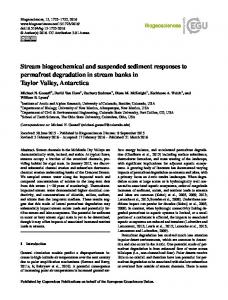
Figure 2-2 Cu data lie on Thompson-Howarth Plot (a model for 10% precision and 95% significant level)

Figure 2-2 shows Thompson-Howarth plot, a precision model, which contains information of the numbers of ‘outlier’ data in duplicate samples for Cu. The value of outlier data lies outside the data range of the precision model. The data are represented by points that fall to above/left of the line. The points represent a pair of duplicate samples whereas the line represent percentile of the half normal distribution (Garrett and Grunsky, 2003; Reimann et al., 2008). In figure 2-2 shows Howarth-Thompson plot for Cu with 5% of RSD value or 10% precision and 95th-tile line. Thompson-Howarth plot for others elements could be seen at appendix 2-3. In addition, table 2-1 is summary of percentage that fall below the 95th-tile line. Thus, as illustration for Cu, the table shows that the value is 80%, it means 20% of the data are lying outside the data range of the model for 10% precision and 5% significant level.

The results from ANOVA, table 2-2, shows that the F-values for all elements are greater than Fc (=1.33). The Fc was determined for 5% in confidence level, 133 and 134 for numerator and denominator degree of freedom, respectively. In addition, regarding the percentage of procedural error value, Zn, Cu, Pb, Ni, Co, Mn, Fe, Hg, Sb, As, Ba, Ce, and Cr have satisfactory results, whereas Ag, Mo and Rb have poor results because their percentages are more than 20%. The Howarth-Thompson plot, in this case, could not be used to determine the reliability of stream sediment geochemical data because all elements have precisions of less than 10%. Thus the reliability of the data was determined by ANOVA test results. Consequently, from the results, there are three elements (Ag, Mo, Rb) were excluded for the next analysis. It is because their procedural error is too large thus their variance could not represent geochemical variance in nature.

15


T Table 2-1 Sum mmary of geoch hemical data quuality asssessment basedd on a Thompson-Howarth Plot (a mo odel for 10% precision p and 95% 9 significant level)

2.4.2.

Table 2-2 Summary of ggeochemical daata quality t assessment based on ANOVA test

Data distrib bution

Histo ogram show that t data disttribution of Zn Z is positively skewed (ffigure 2-3(a)). The same trend happenss for otthers elemen nts of stream sediment geeochemistry (appendix ( 2-4). It means m most of the data d have low w values and distribuution is not symmetric. Th herefore, base-10 logarithmic transform mation was applied a to thee data as suggestedd by Reiman nn et al. (20005) that sttream sedimeent geochem mical data ussually follow w ns. Results off the transforrmation coulld be seen in ffigure 2-4(b), showing thatt logariithmic normaal distribution more symmetric and a less skew wed data disttribution. Hisstogram for logarithmic l ttransformatio on for otherss d o skewness value beforre and afterr of elemeent could bee seen in apppendix 2-4. Significant differences transfformation could be seen at a the last coluumn in table 2-3. 2

166


(a)

(b b)

Fig gure 2-3 Histoggram for Zn, (a) ( graphs for raw r data witho out transformaation, (b) graph hs for base-10 logarithmic transformatio on data Taable 2-3 Univaariate statisticss for stream sediment geocheemical raw datta and skewnesss of base-10 logarithmic transformed d data

2.4.3.

Clustered Images

The algorithm a fro om Raftery and a Dean (22006) and Raaftery (2009) has selectedd nine elemeents from 133 elemeents to be inccluded in Mcclust to get an n optimum clluster numbeer. The nine eelements (Ass, Zn, Cr, Ce,, Ba, Sb b, Fe, Co, Nii) will be called Selected Elements. E Th hese selected elements werre also emplo oyed in PAM M clusteering to test whether w the clustering c usin ng selected ellements givess better resultts than using all elements. mbers are ob btained from m Mclust forr different datasets d andd Different model types and cluster num n convention nal approach to data prep paration, Model types fittting the data are a VEV-transfformation. In modeel with six cllusters and a VVV-modeel with eightt clusters forr all elementts and selectted elements,, respectively. A VVV-model V w with five cluusters fits thee data in the CoDa app proach. The VEV-modell oidal distribuution, equal shape and varying volumee, shape, and d orientation;; represents clusterss with ellipso V-model represents clustters with elliipsoidal, varyying volumee, shape, and d orientation n whereeas the VVV (Fraleey and Rafterry, 2006). More model types can be seeen in appendixx 2-1. o 15 was tried as an inpuut in PAM cllustering in o order to get an optimum m Clusteer number (k) from 3 to clusteer number wh hich shown by b the highest SC value. However, H SC values for alll datasets do not show an n optim mum SC valuue rather thaan relatively constant. c Th he SC values are steady iin range of 0.10 0 to 0.12.. Accorrding to SC subjective s intterpretation table t from Kaufman K and Rousseeuw ((2005), SC vaalue below orr 177


equal to 0.25 is indicating no substantial structure in the data. Therefore, the same cluster number as an optimum cluster numbers from Mclust for the same dataset was used as an input in PAM clustering. Figure 2-5 shows the results of clustering using Mclust and PAM clustering with two different data preparation approach, conventional and CoDa. In general, the results show prominent cluster patterns for three features, one feature lies on the centre and elongates from north-west to south-east, other lies on the eastern part and the rest lies on the southern part. Moreover, according to existing lithological map (see appendix 1-1), these features might be related to three lithologies which are Intrusive Rocks, Volcanic Rocks and Sedimentary Rocks 4, respectively. Furthermore, figure 2-6 shows final results after post clustering processes (interpolation, rasterizing, reclassification, and filtering) were performed. In rasterizing, a 500 m grid size was selected as a result of compromising among proper grid size according to sample density and memory of R application. Whereas according to equation 2-18 by using density sample (1 sample per 10 km2) as an input, 250 m is obtained as a proper grid size. In addition, generally, the patterns in these final results have the same patterns as the clustering results.

18


(a)

(b)

(c)

(d)

(e) (f) Figure 2-4 Clustering results of stream sediment geochemical data for different clustering techniques and different approaches in data preparation, (a) Mclust with conventional approach for all elements, (b) PAM clustering conventional approach for all elements, (c) Mclust with conventional approach for selected elements, (d) PAM clustering with conventional approach for selected elements, (e) Mclust with CoDa approach, (f) PAM clustering with CoDa approach 19


(a)

(b)

(c)

(d)

(e) (f) Figure 2-5 Results after post clustering (rasterizing, reclassification and filtering) of stream sediment geochemical data for different clustering techniques and different approaches in data preparation, (a) Mclust with conventional approach for all elements, (b) PAM clustering conventional approach for all elements, (c) Mclust with conventional approach for selected elements, (d) PAM clustering with conventional approach for selected elements, (e) Mclust with CoDa approach, (f) PAM clustering with CoDa approach 20


2.4.4.

Quantitativve data quality

Produucer’s accuraacy table sho ows that Mcllust accuracyy is higher th han that of PAM clusterring in mostt litholo ogies (figure 2-7). 2 Lithologgies A, B and F have moderate to high accuracies fo or most clusttering results.. Thesee results are consistent with w visual in nterpretation of clusterin ng results thaat show threee prominentt featurres that are related r to Vo olcanic Rockss, Intrusive Rocks R and Seedimentary R Rocks 4. For Lithology C,, the Sedimentary S R Rocks 1, thee accuracy is low for mo ost clusteringg results. Thiis might be because thiss litholo ogy lies beneeath Williston n Lake and is surrounded by b another an nd more abun ndant Sedimentary Rockss 4 thus its geochem mical signaturre was covereed. Accorrding to tablee 2-4, Mclust is better than n PAM clusttering when clustering c usiing both all elements e andd selectted elements.. Clustering number, n as in nput in PAM M clustering, might be on ne of the factors why thee accuracy of PAM clustering is lower compaared to Mcluust. As explain ned in the prrevious paraggraph, the SC C values for PAM clustering c are not indicatin ng an optimuum number of o clusters. IIn addition, the t table also o descriibes that the clustering ussing selected elements pro oduces a sligh htly higher acccuracy than using all thee elemeents. Howeveer, the Kapp pa coefficien nt for PAM clustering ussing all elem ments is little higher than n clusteering using seelected elemeents. Thus, itt is hard to say that clusteering using seelected elemeents is betterr than using all elem ments. Furth hermore, in regard r to data preparatio on, CoDa approach resullted in lowerr accuracy for Mcluust but higherr for PAM cluustering com mpared to the conventionaal approach. Furthermore, F , ppropriate usiing conventio onal approach h, whereas fo or PAM clusttering, CoDa is preferablee Mclusst is more ap to con nventional ap pproach. How wever, accordding to the Kappa K coefficiient value forr PAM clusteering, there iss no siggnificant diffe ference in thee value betweeen using con nventional andd CoDa apprroach in dataa preparation.. This suggests thatt the data aree likely not to oo much affeected by the closure prob blem. It migh ht be becausee he total conceentrations off stream sediiment geochemistry is less than 5%. The closuree the avverage of th probllem arises wh hen total conccentrations of elements ap pproaches k, in this case 1100%.

Figurre 2-6 Produceer’s accuracy diagram d from assessment a of clustering resuults for stream m sediment geo ochemical data (fo or error matricces see appendixx 2-5); Lithologgy A, Volcanicc Rocks ; Litho ology B, Intrussive Rocks ; Liithology C, Sedimentary Rocks R 1; Lithollogy D, Sedim mentary Rocks 2; Lithology E, E Sedimentaryy Rocks 3; Lith hology F, Sedimeentary Rocks 4 (for explanattions about thee lithology at th he study area ssee section 1.6.22)

21


Table 2-4 Data quality of clusstering results for stream seddiment geocheemical data

2.5.

Concludin ng remarks • Conveentional apprroach in datta preparation stage is plausible p to b be employed d for stream m sedimeent geochemiical data with h low total ellements conccentration beefore the app plication such h clusterring methods. • Clusterring using selected s elem ments in streeam sedimen nt geochemiical data pro oduces non-significcant accuraciies. The accuracies are inccreasing only 1% and andd 0.02 for oveerall accuracyy and kaappa coefficieent, respectively. • The ap pplication off Mclust to sttream sedimeent geochemiical data classsification pro oduces betterr accuraacies than thee application of o PAM clustering in mosst assessmentt including th he producer’ss accuraacy for most lithologies l (seee figure 2-6 an nd table 2-4).

222


3.

AIRBORNE GAMMA-RAY DATA ANALYSIS

3.1. Introduction Similar to chapter 2, in this chapter two applications were tested which are the application of different clustering techniques and the application of compositional data (CoDa) approach. Like in the previous chapter, two clustering algorithms, model-based clustering, Mclust and distance-based, PAM (Partition Around Medoids), were performed. Furthermore, conventional and CoDa approach were applied in the data preparation stage. 3.2. Descriptions of the Airborne Gamma-ray Dataset The airborne radiometric data used in this research were downloaded from the National Gamma-Ray Spectrometry Program (NATGAM) Data Base from the Geological Survey of Canada website (Natural Resources Canada, 2010b). Data on concentrations of radioelements (K, eTh, and eU) are available in 250 m grid size. K concentration is measured in percentage (%), whereas eTh and U are in parts per million (ppm). The data are the result of several hundreds of airborne surveys of the Geological Survey of Canada for over 30 years since 1970. The aircraft flew along a pattern of parallel flight lines at 120 m terrain clearance with line spacing 200-500 m. The aircrafts flew at speed around 190 km/h. The data were acquired by sampling every 1 second interval, which equivalent around 60 m on the ground (Natural Resources Canada, 2010b). 3.3. Methodology The methodology described in this chapter could be divided into several stages such as data preparation, clustering, post clustering and assessments. In data preparation stage, two approaches, conventional and CoDa approach, were applied for comparison. Furthermore, two types of clustering techniques were applied for data classification, Mclust and PAM clustering. The post-clustering comprises reclassification and filtering. The assessment is the last stage, which was employed after post-clustering reclassification was conducted. The flow chart of the methodology can be seen in figure 3-1. 3.3.1.

Data preparation

Univariate graph such as histogram was used to investigate element data distribution. For examining spatial distribution, a visualization of element concentration data to an image is quite useful to get an impression of the spatial data distribution. In addition, square-root transformation was chosen to be applied according to the smallest skewness value (Reimann et al., 2008; Weisberg, 2005). For standardization, median-MAD (median absolute deviation) standardization was applied to transformed data (equation 2-10). Transformation and standardization were conducted to get a symmetric data distribution shape and comparable range values as suggested by Reimann et al. (2008) and Templ et al. (2008). In the CoDa approach, several processes were applied in data preparation stage such as data transformation. The first process was converting the data into the same unit of measurement. In this case, K concentrations were converted form percentage into ppm. The three radioelement concentration data from airborne gamma-ray surveys are considered as sub-composition data; thus, they are subjected to the closure operation using equation 2-13. Then, the isometric log ratio (ilr) transformation, equation 2-4, was also applied before the applications of cluster analysis algorithms.

23


3.3.2.

Clustering

Two types of clustering algorithm, Mclust and PAM clustering, were applied to the data for classification. An optimum cluster number for PAM clustering is determined by the highest value of SC (or Silhouette Coefficient); whereas for Mclust, the number is determined by the algorithm based on the highest BIC (or Bayesian Information Criterion) value (see section 2.2.3.1).

Figure 3-1 Flow chart of methodology to map lithology using airborne gamma-ray datasets by applying two types of clustering algorithm, Model-based Clustering (Mclust) and Partition Around Medoids (PAM) clustering with two approach in data preparation stage, conventional and compositional data (CoDa)

3.3.3.

Post clustering

Reclassification and filtering were conducted in sequence after clustering algorithm was applied to the data. Reclassification is needed to make cluster number the same as the reference features for validation whereas the purpose of filtering is to eliminate small or individual cluster. Reclassification using majority rules and majority filtering were performed before the assessments as explained in chapter 2. 3.3.4.

Assessments

Error matrix and kappa coefficient were calculated to assess quality of classification results from Mclust and PAM clustering. The clustering results were compared to reference data which is a simplified existing lithological map (appendix 1-2). From the error matrix, the overall accuracy and producer’s accuracy was calculated to assess the classification outcome. Furthermore, the kappa coefficient, as an indicator to estimate true agreement of classification from the percentages of an error matrix, was also calculated (Lillesand and Kiefer, 2000).

24


3.4.

Results and a discussio ons

3.4.1.

Data distrribution of airb borne gamma-ray elements

Histo ogram in figurre 3-2 (a) show w that data distributions d thereof t K data is positiveely right skew wed. Appendixx 3-1, data d distributtion for eTh and eU, sho ow the same event as thaat of K. The event descriibes that low w conceentration of the elemen nts is more dominant th han high co oncentration. Consequenttly, the dataa distrib butions have asymmetric shape. Thereefore, square--root transformation was performed to t the data in n orderr to get morre symmetricc data distrib bution. The transformatio t on was chossen base on the smallestt skewn ness values. The T transform mation reduced skewness values more than eight tiimes in average comparedd to skeewness valuees before tran nsformation (table 3-1). Fig igure 3-2 (b) an nd appendix 33-1 visualize that t after thee transfformation, th he data distrib bution is morre symmetric.

(a) (b b) Figu ure 3-2 Histoggram for potassium (K), a) hiistogram for raaw data, b) hisstogram after ssquare-root traansformation Table 3-1 Un nivariate statistiics summary for fo airborne gamma-ray raw data d and its skkewness of squuare-root d data transformed

255


(a)

(b) Figure F 3-2 sho ow spatial diistribution variation v for th he three radio oelement dattasets. The im mages reveal th hat the upperr central of tthe area (sym mbol x in the im mages) all eleements have high concentration. The prominent p co oncentration might be rellated to the Syenite S Form mation. Syeniite contains K-rich and Na-rich N feldsp par as well aas high in U (Wilford et al., 1997). Another A simiilarity is thaat the lake ( appendix feeatures couldd be distinguiished easily (see 1-2). The im mages show w that in general, g the so outhern partt of the area has lower raadioelement concentration n than the no orthern part. It might be Rocks, at the north, that reelated to thee Intrusive R higher raadioelement reelatively h have a concentration n to sedimen ntary rock, att the south. ( (c) Furthermore, F in general, T Th and U haave a similar Figure 3-3 Spatiial data concen ntration distrib bution of sp patial concen ntration distri ibution than with w K. It is borne gamma-rray elements (aa) K (%), (b) eTh e (ppm) airb because b Th a and U have converse ch haracteristic and (c) eU (p ppm) with h K such as in i weatheringg and minerallization. Nevvertheless, sp patial distribuution of U is more m erratic as can c be seen at a eastern paart. The heterrogeneous sp patial distribuution of U is understandaable because thiss element is more m easily in nfluenced byy weathering and mineraliization than K and Th (D Dickson and Sco ott, 1997; Willford et al., 19997). 3.4.2.

Clustered d images

Appliication of Mclust to radio olement dataa based on different d apprroaches in ddata preparatiion producess differrent models (figure (f 3-4(a) an nd figure 3-4(c (c)): a VVV-m model with nin ne clusters an nd a VEV-mo odel with fivee clusteers are the mo odels obtaineed after appliication of con nventional an nd CoDa dataa preparation n approaches,, respectively. The VVV-model V represents clusters c with ellipsoidal, vaarying volum me, shape, and d orientation n in feaatures spaces; whereas the VEV-model representss clusters witth ellipsoidal distribution, equal shapee and varying v volum me, shape, an nd orientation n (Fraley and d Raftery, 20006). More mo odel types caan be seen in n appenddix 2-1. SC vaalues using a cluster numb ber (k) from 3 to 15, as an a input in PA AM clusterin ng, are rangin ng from 0.21-0.30. The highestt numbers obtained o at k =3, howevver the clusteer result is ttoo general when it wass visuallized. Thereffore, the sam me cluster numbers as an a optimum cluster num mbers from Mclust, M weree selectted to get mo ore clusters ass shown in figgure 3-4(b) and d figure 3-4(d). i for CoDa C approaach (figure 3-44(c) and figure 3-4(d)) have more isolateed and smalll Clusteering result images clusteers than those of conventtional transfo ormation (figuure 3-4(a) and figure 3-4(b)). The small clusters c couldd be seeen at the north-eastern n n part of th he area. The images couuld not iden ntify the areea, where alll 266


radioelements have high concentrations as clearly seen in figure 3-3, and the lake features. However, an area at the southwest is more homogeneous in the results of CoDa approach than those in the results based on the conventional approach. After post clustering processes were conducted, all images show that a consistency in identifying some particular features. For example, the images could give perceptions about the boundaries between sedimentary rocks and volcanic rocks as well as sedimentary rocks and intrusive rocks. Moreover, the area at the centre of the area, which contains high concentrations of K, eTh and eU, which might be related to occurrence of Chuchi Syenite Formation, could be detected in most images. This area might be. However, the algorithms failed to differentiate between volcanic rocks and intrusive rocks at north western and eastern part respectively (figure 3-4). The above results are consistent with the references that explained about the confusion in differentiating among volcanic rocks, intrusive rocks. This could be due to count levels of volcanic rocks is much lower than those of the intrusive units (Graham and Bonham-Carter, 1993).

(a)

(b)

(c)

(d)

Figure 3-4 Clustering results of airborne gamma-ray data for different clustering techniques and different approaches in data preparation, (a) Mclust with conventional approach, (b) PAM clustering conventional approach, (c) Mclust with compositional data approach, (d) PAM with compositional data approach

27


(a)

(b)

(c)

(d)

Figure 3-5 Results after reclassification and filtering of airborne gamma-ray data for different clustering techniques and different approaches in data preparation, (a) Mclust with conventional approach, (b) PAM clustering conventional approach, (c) Mclust with compositional data approach, (d) PAM with compositional data approach 3.4.3.

Quality of the classification

Figure 3-6 show that producer’s accuracy of Mclust with conventional approach is the best among the others clustering algorithms because its consistency. The results have a moderate accuracy for Feature B (Intrusive Rocks) and Feature C (Sedimentary 1), in which others clustering have a low accuracy. The relative low accuracy for Feature B is due to confusion between Volcanic and Intrusive Rocks as explained in previous paragraph. For Feature C, this might be due to the fact that its areas are small and surrounded by Volcanic Rocks thus its radiometric signature become unclear. Mclust accuracies are higher about 15% than those of PAM clustering as shown in table 3-2. The producer’s accuracy of Mclust is relatively higher for most lithologies than that of PAM clustering. Its low accuracy due to the algorithm does not find a substantial structure in the data. When no a substantial structure finds, the results is becoming less representative to be use for explaining the processes/phenomena in the area where the data are taken. Regarding the data preparation approach, CoDa approach does not produce better classification results compared to the conventional one (table 3-2). Classification accuracy based on CoDa is lower than that based on the conventional one with more 15% and 25% differences for overall accuracy and kappa 28


coefficient, respectively. In addition, figure 3-6 a diagram of producer’s accuracies, shows that the conventional approach produces better results than CoDa. It might be due to the fact that total concentrations of K, eTh, and eU are only less than 5%, as explained by Pawlowsky-Glahn and Egozcue (2006) that closure problems arise when the sum of data per sample approaches the constant k (k = 100% or k = 1,000,000 ppm in this case). Therefore, CoDa approach likely is not appropriate to be applied in this type of data. The moderate to low level accuracy of clustering results might be influenced by input data and the field condition. The input data are not primary data but were already in grid format, and we know that gridded data are interpolated data. Consequently, interpolation errors contribute to the total error of the assessment. According to field conditions, the area is heavily weathered and covered by a thick layer of sand and gravel left behind by glaciers (Geoscience BC, 2010). Consequently, the boundaries from clustering results have a low accuracy compared to the reference existing lithological map.

Figure 3-6 Producer’s accuracy diagram from assessment of clustering results for airborne gamma-ray data (for error matrices see appendix 3-2); Feature A, Volcanic Rocks; Feature B, Intrusive Rocks; Feature C, Sedimentary Rocks 1; Feature D, Sedimentary Rocks 2; Feature E, Lake (for explanations about the lithology at the study area see section 1.6.2) Table 3-2 Data quality of clustering results for airborne gamma-ray data

29


3.5.

Concluding remarks • The clustering method could be used to recognize lithologies with distinctive characteristics and/or large homogenous areas. Lithological units with distinctive characteristics, e.g. high concentration in gamma-ray elements such as Chuchi Syenite formation, are prominent in almost all clustering algorithm. Furthermore, a large homogenous area such as Sedimentary Rock 2 also could be identified (see figure 3-6). • CoDa approach in data preparation likely is not a proper technique to be applied in airborne gamma-ray that shown by its lower accuracies (see table 3-2).This might be because the closure problems are insignificant in the data. • Classification qualities of Mclust to airborne gamma-ray data are better than these of PAM clustering with the differences up to 7% and 0.09 for overall accuracy and kappa coefficient, respectively.

30


4.

AIRBORNE MAGNETIC DATA ANALYSIS

4.1. Introduction In this chapter, edge detection methods – rotation-variant template matching (RTM) and clustering-based for edge detection (CED) – were applied to identify lithology boundaries from airborne magnetic data. The methods were chosen rather than region-based segmentation due to characteristics of magnetic data. Magnetic data have non uniform value rather than gradual value even within one lithology. Thus edge detection is more suitable because the methods detect abrupt change in the values not their similarity such in region-based segmentation. Furthermore, before application of these techniques, two common transformations in analyzing magnetic data – reduce-to-pole (RTP) and analytic signal (AS) – were applied as data preparation methods. The results were used to interpret lithological boundaries. The interpretations are to be used in chapter 5 for assessing classification accuracy. 4.2. Descriptions of the Airborne Magnetic Datasets Airborne magnetic data (residual total magnetic intensity) were obtained from the Canadian Aeromagnetic Database maintained by the Geological Survey of Canada (Natural Resources Canada, 2010a). The data were obtained from the airborne surveys using the flight-line orientations that were approximately perpendicular to the regional geological strike in constant line spacing. The aircraft flew with 305 m of terrain clearance and 800 m of flight line spacing. The data were available in grid form with 200 m grid size with coordinate system in WGS 1984 UTM zone 10 N and datum of WGS 1984 datum. The residual total magnetic intensity was obtained by subtracting from the observed total field the International Geomagnetic Reference Field (IGRF) model (Natural Resources Canada, 2010a). 4.3. Methodology Two techniques of edge detection were applied to the airborne magnetic data in order to identify boundaries between lithological units. Rotation-variant template matching (RTM) algorithm developed by (Van der Werff et al., 2007) and clustering-based for edge detection (CED) algorithm developed by (Dinh et al., 2009) were applied to the airborne magnetic data after some data preparation processes were performed to these data (figure 4-1). RTM algorithm was applied to a subtraction image whereas CED was applied to the horizontal derivative image. It is because the two algorithms have a difference in defining the edge. RTM defines the edge as an area among the areas which have at least two contrasting characteristics e.g. spectral, texture whereas CED define as an area where there are abrupt changes of the characteristics. RTM was applied using ENVI software with ESA Tools add-ons which developed by Department of Earth System Analysis-ITC, whereas k-means clustering, the last part of CED algorithm, was applied using R statistic software with stats package. In addition, the rest of the processes such as in data preparation were conducted using Oasis Montaj 7.2.1 4.3.1.

Data preparation

For comparison, two transformations – reduce to pole (RTP) and analytic signal (AS) – were applied to the airborne magnetic data before the application of the edge detection techniques. As it is shown in figure 4-1, after RTP or AS transformation, upward continuation (UC) was applied to each image. The last process in preparation stage is raster/grid subtraction of RTP and AS image by their UC. The results of their subtraction are so-called RTP subtraction (RTPSub) and AS subtraction images (ASSub), respectively. Subtraction images are another approach to separate between information derived from depth surface and near-surface. As we know that UC transformation tries to attenuate high-frequency signals than low-frequency signal. The high frequency is mostly derived from shallow source (Milligan and Gunn, 1997). Therefore, subtraction images describe more shallow surface anomalies signal.

31


Figure 4-1 Flow chart of the methodology with two different transformations, RTP and AS; and techniques, RTM and CED 4.3.1.1.

Reduce To Pole (RTP)

Figure 4-2 A magnetic anomaly profile and its relation to geological features, before and after being reduced to the pole (Blakely, 1996)

4.3.1.2.

Milligan and Gunn (1997) defined reduce-topole (RTP) as the process to convert the magnetic field from a magnetic at particular latitude to the field at a magnetic pole, where the inducing field is vertical. At a magnetic latitude, magnetic anomalies due to induction have asymmetric form (skewed form) related to their sources, but when the inducing field is vertical the induced anomalies are directly over their sources as shown in figure 4-2 (Blakely, 1996).

Analytic Signal (AS)

AS is a linear combination of first derivatives of magnetic anomaly in horizontal and vertical directions (Roest et al., 1992). The AS has a form over causative bodies that depend on the locations of the bodies but not on their directions of magnetization. This means that all bodies with the same geometry have the same analytic signal. The analytic signal peaks over the edges of source bodies of positive and negative anomalies and thus can be used to determine edge locations (Milligan and Gunn, 1997). 4.3.1.3.

Upward Continuation (UC)

Upward continuation transforms the potential field measures on one surface to the field that would be measured on another surface farther from all sources. This transformation attenuates anomalies with 32


respect to wavelength; the shorter the wavelength the greater the attenuation. This upward continuation tends to emphasize anomalies caused by deep sources at and to reduce of anomalies caused by shallow sources (Milligan and Gunn, 1997). 4.3.1.4.

Subtraction Image

Subtraction image describes signal of magnetic anomaly from shallow sources because it is a result of subtraction between responses signals from all-depth sources anomalies and these of deep-source anomalies. Responses signals from all-depth sources anomalies represent by transformed of residual total magnetic intensity (RTP and AS image) whereas responses signals from deep-source anomalies represent by UC images. Therefore, there are two subtraction images, one is RTP transformed subtraction image (RTPSub) and another is AS transformed subtraction image (ASSub). 4.3.2.

Rotation-variant Template Matching (RTM)

RTM algorithm was applied to the subtraction image both for RTP transformation (RTPSub) and AS transformation (ASSub). The first step to apply the method is determining region of interests (ROIs) to assign into template. The ROIs consist two areas considered representatives of different lithologies. Van der Werff et al. (2007) explained that the template is a miniature image which consists of 3x1 pixels. The template contains information about a boundary between two contrast pixels. These two contrast pixels represent two different lithologies. This template is moved over the image like a moving kernel. At every position, the template is rotated, and a statistical fit is calculated for every pose (Figure 4-3). The next steps are choosing one result from 12 results which produced by the algorithm. Then, the Figure 4-3 Template is matched by (a) moving it over threshold value is determined base on natural an image and (b) changing the template orientation at breaks using Jenk’s optimization (Jenks, 1967). The every position by 45° increments up to a total of eight orientations (Van der Werff et al., 2007) threshold divides the data into edge and non-edge pixel. The algorithm, in principle, tries to minimize the variance within the classes and maximize and maximize the variance between the classes. The natural breaks technique was used when the data is not evenly distributed and not heavily skewed toward one end of the distribution. 4.3.3.

Clustering-based Edge Detection (CED)

Clustering-based edge detection (CED) algorithm from Dinh et al. (2009) for edge detection was applied to the airborne magnetic data. The algorithm consists of several steps as follow: first, Gaussian blur convolution was applied to the subtraction image (RTPSub or ASSub) to reduce the noise in order to avoid local anomalies when horizontal derivative was applied. The horizontal derivate was employed to get gradient image in lateral direction. The step was needed due to the algorithm is looking for sudden change of value. The next step is applying k-means clustering to the gradient images. Dinh et al. (2009) suggested cluster number four to eight to be tried as an input in k-means clustering. Whereas two clusters is not recommended because the pixel values tend become non-edge cluster thus there is possibility to loss edge clusters. The next step is distinguishing clusters into edge and non-edge cluster base on pixel number of cluster members. Two clusters with the highest pixel number were classified into non-edge cluster and the rest were into edge cluster.

33


4.4. Results and discussion Figure 4-4 and figure 4-5 show the results of data preparation for RTP and AS transformation part, respectively. Figure 4-4(a) is a result of RTP transformation with 20.3° and 74.9° for geomagnetic inclination and declination, respectively. The values of inclination and declination were generated by Oasis Montaj 7.2.1 with latitude and longitude of the area as well as the time of data acquisition as the inputs. In addition, figure 4-5(a) is a result of AS transformation. In both images, the features have the same pattern which is north-west to south-east trending. From both images, the area with high values in RTP is wider than these in AS. This is might be due to remnant magnetization in the area. As explained by Milligan and Gunn (1997), the remnant magnetization could smear the anomaly. Figure 4-4 (b) and figure 4-5(b) are the results of upward continuation at an equivalent plane level of 500 m. Both images have smoother images compare to their parents (figure 4-4(a) and figure 4-5(a)). It is because UC transformation smooths out short-wavelength anomalies relative to long-wavelength. The same as their parent, UC from RTP have wider area in high value than that from AS for the same reason. The last two images in figure 4-4 and figure 4-5 are subtraction images and horizontal derivatives or horizontal gradient images. These subtraction images depict the anomaly from shallow sources at the area. Figure 4-4(c), RTPsub, shows wider area for high value than figure 4-5(c), ASSub. This is because the influence of their parent images, which have the same phenomena, is still remained. Both these images were used as input in RTM algorithm. Furthermore, figure 4-4(d) and figure 4-5(d) are horizontal derivative of subtract images that show change intensity of subtract images value. The horizontal derivatives of RTP transformation images show more continuous features than that of AS. However, the AS one has clearer separation between the high value area and its surrounded. In addition, CED algorithm was performed to these images. Figure 4-6 show the results of application edge detection method to airborne magnetic data. Figure 4-6 (a) and figure 4-6 (b) are the result of Frank Ratio 2 image of RTM algorithm for RTP and AS transformed part, respectively. The images have been classified using natural break optimization of Jenk’s algorithm in ArcGIS 10. Frank ratio was chosen because the edges are seen the most clearly in the images. The Frank Ratio 2 is a ratio between rotation variance in mean spectral fit and rotation average spectra variance. The rotation variance in mean spectral fit could be used to indicate existence of crisp boundaries. In addition, the rotation average spectra variance have high value when at least one of the spectral signatures is found and forms a crisp boundary (Van der Werff et al.,2007). Thus, the ratio could be used to indicate crisp boundaries. In general, all results produce the same edge patterns trend, north-west to south-east trend (figure 4-6). This trend is the same as general trend of lithologies and lineament in existing lithological map. However, results of CED are better than RTM because RTM creates multiple responds for a single edge for some parts. Between CED for RTP transformed and AS, it is difficult to assess which one is better. Nevertheless, the image of AS is more reliable when input data, figure 4-4 (a) and figure 4-5 (a), are included as consideration. Therefore, this image was chosen for updating the lithological map. The edge pixels can be distinguished as lithological edge and non-lithological edge that reflect lithological boundaries and lineament signatures, respectively (figure 4-7). The lithological edge is defined as the most outside pixels of clustered edge pixels thus edge pixels within cluster and individual edge pixels are classified to non-lithological edge. From figure 4-7, clustered edge pixels, thus as well as the lithological edges, are only related with the particular intrusive rocks, the Hogem Batholiths. Therefore, the lithological could be used to update of Hogem Batholith boundaries as shown in figure 4-7 (a). The clustered edge pixel in Hogem Batholith might be related to the complex processes of its formation. As explained by Nelson et al. (1992), Hogem Batholith occurred in at least three phases that each create complex features. Thus, to describe its complexity, Hogem Batholith is called as an intrusive complex.

34


(a)

(b)

(c)

(d)

Figure 4-4 Results of processing of airborne magnetic data; (a) reduced-to-pole (RTP), I=20.3°, D=74.9°; (b) upward continuation of RTP at 500 m (UC); (c) RTP subtraction image (RTPSub), RTPS=RTP-UC; (d) horizontal derivative of RTP subtraction image

35


(a)

(b)

(c)

(d)

Figure 4-5 Results of processing of airborne magnetic data; (a) analytic signal (AS), (b) upward continuation of AS at 500 m (UC), (c) AS subtraction image (ASSub), ASS=AS-UC, (d) horizontal derivative of AS subtraction image

36


(a)

(b)

(c)

(d)

Figure 4-6 Images of edge detection technique results, (a) result for RTM technique with RTP transformation, (b) result for RTM technique with AS transformation, (c) result for CED technique with RTP transformation, (d) result for CED technique with AS transformation

37


(a)

(b) Figure 4-7 In nterpretation of clustering-baased for edge detection d (CED D) result base on analytic siggnal (AS) transsformed horizo ontal derivativves images, (a) an existing lith hological map is underlying tto the interpreetation result; dash--thick-lines aree boundaries of o the new inteerpretation, (b) the final resullts of new inteerpretation lith hological map; dash-line box b is the area for assessing classification c a accuracy in chappter 5

4.5.

Concludin ng remarks • The ap pplication of AS to residdual total maggnetic intensiity data in daata preparatio on before thee applicaation of edgee detection methods m is mo ore reliable th han RTP duee the fact thaat AS is moree robustt to the existeence of remnaant magnetization. • CED could becom me an alternaative unsuperrvised technique for classsifying airborrne magneticc data to o indicate thee edge featurees such as lith hological bouundaries and llineaments.

388


5.

STREAM SEDIMENT GEOCHEMICAL AND GEOPHYSICAL DATA INTEGRATION

5.1. Introduction In this chapter, stream sediment geochemical (SSG) data and airborne gamma-ray (AGR) data were integrated by using them as inputs in two different clustering methods – model-based clustering (Mclust) and partition around medoids (PAM) – for unsupervised lithological classification. In the assessment stage, not only the existing lithological map was used to validate the clustering results but also the lithological map based on the interpretation of airborne magnetic data in chapter 4. In addition, accuracies of clustering the SSG data (chapter 2) and the AGR data (chapter 3) were compared to the accuracies of clustering the SSG and AGR data together. 5.2. Datasets for integration study The SSG data consist of 2,194 sampling points for 13 elements, from which nine elements have been selected using the BIC (Bayesian Information Criterion) in order to get the optimum number of clusters (see section 2.3.3.1). The 13 elements are As, Zn, Cr, Ce, Ba, Sb, Fe, Co, Ni, Cu, Mn, Hg, and Pb; the first nine elements were the ones selected using the BIC. The stream sediment sampling density varied from about 1 sample per 8 km2 to 1 sample per 13 km2 (Jackaman and Balfour, 2008). Figure 5-1 shows the study area for the integration of SSG and AGR data. This area is the same as study area for the AGR data only (see figure 1-2 and chapter 3). For SSG data preparation, all the stream sediment sample data (see figure 2-4 for location map) were used in data processing such as interpolation. Then, in integration phase the processed SSG data were subset to the study area for the analysis described in this chapter (figure 5-1). Furthermore, two lithological maps were used for validation of the results. One map (figure 5-1(a)) is the existing geological map that that was used for validating the clustering results using the AGR data (see chapter 3). The other map (figure 5-1(b)) is the result of analysis and interpretation of the airborne magnetic data (see figure 4-7 (b)).

(a)

(b)

Figure 5-1 The study area and maps used for validation of results: (a) existing lithological map; (b) lithological map based on the interpretation of airborne magnetic data, see figure 4-7 (b) (modified from Massey et al. (2005a, b, c, d))

39


5.3. Methodology The integration of SSG and AGR data consist of four stages, namely: data preparation; data integration using clustering method; post clustering; and assessment (figure 5-2). Data preparation comprises of data transformation and standardization of SSG data, and then their interpolation in order to convert the point SSG data into a continuous data layer like the AGR data. The interpolation of the SSG data was performed using ArcGIS 10, whereas variogram analysis before interpolation and clustering analyses were executed using R statistical software. Like in chapter 2 and chapter 3, two clustering algorithms – Mclust and PAM – were performed to integrate the SSG and AGR datasets. Post clustering processes such as reclassification and filtering were employed before the assessments. From the error matrix, overall and producer’s accuracy and kappa coefficient were calculated to assess the classification results. The assessments were conducted using the two reference maps shown in figure 5-1. 5.3.1.

Data preparation

To investigate the spatial data structure of the geochemical data for each element, variogram analyses were performed (appendix 5-1). The variogram models and the point geochemical data were used to interpolate unsampled areas using universal kriging. As explained by Carranza (2010), interpolation is a plausible technique to make continuous geochemical landscapes from stream sediment geochemical data in regional scale. Furthermore, Robinson et al. (2004) stated that universal kriging is an appropriate technique to interpolate stream sediment geochemical data in regional scale. Data transformation and standardization were then applied to the SSG data before clustering techniques were applied. Base-10 logarithmic and square root transformation were applied to the SSG and AGR data, respectively, to get symmetric shape in data distribution. The transformations were chosen according to the skewness values of individual datasets as explained in chapter 2 and chapter 3. In addition, the standardization using median-MAD (equation 2-10) was applied to both datasets to make the range of the data comparable. 5.3.2.

Clustering

Mclust and PAM clustering methods were applied to stacked raster images of SSG and AGR data. As experiments besides using all 13 elements in the SSG data, clustering was also applied to the nine selected elements in the SSG data. Thus, there are two data integration results: Integrated Data I is from combination of SSG all elements with AGR elements and Integrated Data II is from combination of SSG selected elements with AGR elements. 5.3.3.

Post clustering

For the post clustering stage, reclassification and filtering were applied to images of clustering results. The images were reclassified into five classes representing five features as in the reference maps (figure 5-1). Furthermore, before the assessments, majority filtering was applied to the reclassified images. 5.3.4.

Assessments

Two lithological maps, figure 5-1(a) and figure 5-1(b), were used to validate the images resulting from the clustering analyses. The map in figure 5-1(a), the existing lithological map, was designated as Reference Data I, whereas the map in figure 5-1(b), derived from the interpretation of airborne magnetic data in chapter 4, was designated as Reference Data II. This latter reference data were used to test if interpreted lithological boundaries from analysis of airborne magnetic are consistent with results of clustering the SSG and AGR data together. If assessment results using Reference Data II are better than those using Reference Data I, it means that the lithological boundaries interpreted from the airborne magnetic data might be better than those portrayed in the existing lithological map. Furthermore, overall and producer’s accuracy from error matrix and kappa coefficients were used to assess the quality of the classification results.

40

Figure 5-2 Flow chart of the methodology to integrate stream sediment geochemical and airborne gamma-ray data using two types of clustering algorithm, Model-based Clustering (Mclust) and Partition Around Medoids (PAM) clustering.


41


5.4. 5.4.1.

Results and discussion Interpolated images

Figure 5-3 and table 5-1, respectively, show the variogram model for Zn and summary of variogram components for 13 elements in the SSG dataset. A model was chosen based on the smallest root mean square values from three variogram models which had been tried, exponential, gaussian and spherical. The variogram model show spatial data structure of the element at the study area. All the elements data fit with the exponential model that means the data have high variance change within small distance. The range values, the last column of table 5-1, show maximum distance at which the samples still have spatial correlation. Therefore, the models are reliable to be used due to the fact the smallest distance between the samples at the study area are less than 500 m. The variogram models for the other elements in the SSG dataset are given in appendix 5-1. In addition, figure 5-4 shows the spatial distribution of Zn as a result of universal kriging interpolation; whereas maps of spatial distributions of the other elements are shown in appendix 5-2. Table 5-1 Summary of variogram components of individual elements in the SSG dataset

Figure 5-3 Exponential variogram model for logarithmic base-10 transformed Zn data

Figure 5-4 Image of spatial distribution of Zn as a result of universal kriging 42


5.4.2.

Clustered images

Figure 5-5(a) is an image of Mclust results using SSG and AGR data together (Integrated Data I). The best model for the data base on BIC is an EEV-model with nine clusters. This model means that the nine clusters have equal volumes and shapes but vary in orientations of ellipsoidal distributions in feature space. In addition, the image depicts several homogenous clusters with clear separation between them. For PAM clustering, the optimum cluster number for Mclust for the same data was taken as an input. It is because values of SC (Silhouette Coefficient; see section 2.3.3.1) in PAM clustering for cluster number (k) from 3 to 15 did not show an optimum cluster number but rather fluctuate at a constant range between 1.3 to 1.5. According to Kaufman and Rousseeuw (2005) when the SC value is below 0.25, it means that there is no substantial structure in the data as shown in appendix 2-2. When there is no substantial in the data, the data using this technique become less reliable to be used to explain the processes/phenomena. Furthermore, figure 5-5(b), the result of PAM clustering using Integrated Data, shows several clusters with clear boundaries among them and several individual clusters within them. However, the PAM clustering image shows that lake boundaries could be detected quite well as can be seen in figure 5-5(b). Figure 5-5(c) and figure 5-5(d) are the images resulting from clustering using the nine selected elements in the SSG data and the AGR data (Integrated Data II). These images show similar patterns as their corresponding resulting from Integrated Data I. For Mclust, the same model as for Integrated Data I, an EEV-model with nine clusters, was also obtained. In addition, PAM clustering used the same cluster number from the Mclust result as an input in the process. The number was taken due to the difficulties in determining an optimum cluster number based on SC. Comparing images resulting from Mclust, figure 5-5(a) and figure 5-5(c), with those resulting from PAM clustering, figure 5-5(b) and figure 5-5(d), reveals that the clusters of Mclust are larger and more homogeneous than those of PAM clusters. Furthermore, it is apparent that Mclust is a better technique than PAM clustering in distinguishing large features such as both sedimentary rocks. However, PAM clustering could detect small features, such as lakes, better. Figure 5-6 and figure 5-7, which are results of reclassification and filtering, demonstrate that patterns of particular clusters are similar to patterns of particular feature in reference data. Both figures have similar patterns, except for Intrusive Rocks. It is due to the facts that figure 5-7 using Reference Data II as a basis for reclassification. As explained in previous section, the Reference data II data is a lithological map base on airborne magnetic data analysis which updating new boundary for Intrusive Rocks. Furthermore, for example, in figure 5-6(a), pattern of Cluster D is similar to that of the Sedimentary Rocks 2 in southwestern parts of the areas. This pattern is found also in figure 5-6(c), and figure 5-6(d), whereas for figure 56(b) the pattern is somewhat elongated to the east. Besides the pattern of Cluster D, in figure 5-6(a), the pattern of Cluster A is also similar to that of Intrusive Rocks in the existing lithological map. Moreover, among all images, figure 5-5 (a) has the clearest boundaries of lithological units, except for the lake features. Like in figure 5-6, in figure 5-7, the sedimentary rocks unit could also be recognized. The same as figure 56(a), Mclust results for Integrated Data I, figure 5-7(a) could identify the Instrusive Rocks and give the most obvious boundaries among lithological units.

43


(a)

(b b)

(c) (dd) Figurre 5-5 Clusteriing results imaage, (a) Mclust for all elemen nts of stream seediment geoch hemical data an nd gamma-ray daata integration,, (b) PAM clusstering for all element e of streeam sediment geochemical ddata and gamm ma-ray data integrration, (c) Mcluust for nine sellected elementt of stream sed diment geocheemical and gam mma-ray data in ntegration, (d) P PAM clusterin ng for nine seleected element of stream sediiment geochem mical and gamm ma-ray data inttegration

444


(a)

(b)

(c) (d) Figure 5-6 Images after reclassification and filtering using existing lithological map (Reference Data I), (a) Mclust for all element of stream sediment geochemical and gamma-ray data integration, (b) PAM clustering for all element of stream sediment geochemical and gamma-ray data integration, (c) Mclust for selected nine elements of stream sediment geochemical and gamma-ray data integration, (d) PAM clustering for nine selected element of stream sediment geochemical and gamma-ray data integration

45


(a)

(b)

(c) (d) Figure 5-7 Images after reclassification and filtering using lithological map based on the interpretation of airborne magnetic data in chapter 4 (Reference Data I), (a) Mclust for all element of stream sediment geochemical and gammaray data integration, (b) PAM clustering for all element of stream sediment geochemical and gamma-ray data integration, (c) Mclust for selected nine elements of stream sediment geochemical and gamma-ray data integration, (d) PAM clustering for selected nine elements of stream sediment geochemical and gamma-ray data integration. 5.4.3.

Quality of classification

Regarding producer’s accuracy, consistent results, in terms of differences among lithological units, are obtained as displayed in figure 5-8. For assessment using Reference I, the consistency could be observed such as for Features A, D, and E. The differences are roughly 10% between the highest and the lowest percentage. Producer’s accuracy for Feature A is roughly the same at 50-60% whereas producer’s accuracy for Features units D and E are higher at 70-80%. In addition, producer’s accuracy for Features B and C is variable depend on clustering type and data preparation. Table 5-2 shows that assessment results vary from 51% to 62% and from 0.3 to 0.45 for overall accuracy and kappa coefficient, respectively. The lowest accuracy of 51% is obtained in PAM clustering of Integrated Data II with respect to both Reference Data I and II. The lowest accuracy, even is still in moderate level, might be due to its low SC value which describe that the data are less representative to depict the process in the area. The highest accuracy is 62% when Mclust clustering was applied into Integrated Data I with respect to Reference Data I as shown in table 5-2 (a). Similar to overall accuracy, kappa coefficient is worse when Integrated Data II was used with respect to both Reference Data I and 46


Reference Data II. In addition, table 5-2 also shows that the assessments using Reference Data I are better than using Reference Data II. According to assessment results, Mclust and PAM clustering have similar accuracy values. However visually, Mclust images are better than PAM clustering images. It is because the cluster patterns from Mclust have similar general patterns as in the existing lithological map except for the lakes features. Thus, for the next research, it is suggested to integrate satellite imagery such as Landsat or Aster imagery in order to identify water bodies such as lakes features. In addition, Mclust result images have more homogeneous cluster areas than PAM clustering images. It might be because in PAM clustering an optimum cluster number was not achieved. 5.4.4.

Comparison of individual data

Producer’s accuracies of integrated data with respect to Reference Data I tend to be similar to the results of using AGR data (chapter 3). It might be due to the influence of sample density and regularity pattern of AGR data. AGR data have denser sampling density than SSG data, the former have density about 1 sample per 0.25 km2 whereas the latter have density of 1 sample per 13 km2. In addition, the pattern of the sample points may also influence accuracy in interpolation results. Furthermore, in interpolating SSG data, it was difficult to find appropriate variogram models when only using SSG data within the integrated/AGR study area; thus, data within the whole stream sediment study area were employed (chapter 2). Producer’s accuracies of integrated data with respect to Reference Data II are not similar to those of only either SSG data (chapter 2) or AGR data (chapter 3). Thus, the interpretation of lithological boundaries based on airborne magnetic data (chapter 4) might not be better than the existing lithological map. It is due to the fact that the similarity signatures between intrusive and volcanic rocks in magnetic data whereas in the field, geologist could differentiate between them. However, there is similarity of pattern for the intrusive lithological unit when comparing between the lithological map based on airborne magnetic data, figure 5-1 (c) and the clustering result base on CoDa for AGR, figure 3-6 (c) and figure 3-7(d). This result needs further investigation whether there is real correlation or it is just due to a chance. Overall accuracies of clustering the SSG and AGR data together are higher than these of SSG and AGR data. However, their better results are inconsistent with respect to producer’s accuracy except for Mclust using combination of SSG all 13 elements with AGR data (Integrated Data I). In addition, when the accuracies of SSG data is compared to these of AGR data, Intrusive Rock could be well detected in SSG data whereas Volcanic Rocks could be well distinguished in AGR data. For other features, accuracy of both data shows almost the same results. Furthermore, producer’s accuracies of Mclust using Integrated Data I have relative a higher or the same as these of SSG and AGR data. The selection elements of SSG data are not produce better results, as shown in chapter 2, when they are combined with AGR data. It might be because structures in SSG data only are different from these in the SSG and AGR data together. Accuracy of clustering results using the integrated data is dependent on spatial data structure. It is because values in the integrated datasets that were used inputs for clustering are interpolated data. The spatial data structure will influence the selection of appropriate interpolation technique. In the case when the data have no spatial structure, interpolation technique such as kriging is not an appropriate technique.

47


(a)

(b) Figure 5-8 Producer’s accuracy diagram from assessment of clustering results (for error matrices see appendix 5-3 and 5-4), (a) an assessment using existing lithological map for the reference (Reference Data I), (b) an assessment using map of the interpretation of airborne magnetic data (Reference Data II); Feature A, Volcanic Rocks; Feature B, Intrusive Rocks; Feature C, Sedimentary Rocks 1; Feature, Sedimentary Rocks 2; Feature E, Lake (for explanations about the lithology at the study area see section 1.6.2)

48


Table 5-2 Comparison of clustering results assessment based on stream sediment geochemical data only, airborne gamma-ray only, and integration of both datasets, (a)accuracy using combination of stream sediment geochemical (SSG) all 13 elements with airborne gamma-ray (AGR) elements (Integrated Data I), (b) accuracy using combination of SSG selected nine elements with AGR elements; *) an assessment using existing lithological map for the reference (Reference Data I), **) an assessment using map of the interpretation of airborne magnetic data (Reference Data II) (a)

(b)

5.5.

Conclusion remarks • Based on the overall accuracy and kappa coefficient, clustering results of integrated data (stream sediment geochemistry and airborne gamma-ray) are higher than those of individual data. • Mclust results are better than PAM clustering results. It is shown by the general pattern similarity of clustering image to existing lithological map. • Mclust technique could be used as an alternative technique in order to integrate stream sediment geochemical and airborne gamma ray data for mapping the lithology in regional scale.

49


6.

CONCLUSIONS AND RECOMMENDATIONS

6.1. Conclusions Base on the research results, the research questions could be answered as follows: Could stream sediment geochemical data (SSG) be used to assist lithological mapping in vegetation-covered areas where no or little a-priori information about underlying rock units is available? Mclust and PAM clustering could be alternatives techniques for classifying stream sediment geochemical data to help lithological mapping in area with limited information. The images of their results depict pattern similarities to the existing litholigical map. In addition, the assessments of the results show moderate accuracy up to 51% and 0.41 for overall accuracy and kappa coefficient, respectively. In addition, for a large homogeneous lithology, the producer’s accuracy is quite high up to 80%. Does the application of compositional data (CoDa) analysis to SSG data and airborne gamma-ray (AGR) data produce better results than conventional methods? In general, the application of CoDa approach in data preparation to both SSG and AGR data do not produce better accuracy than conventional approach. The assessments show the differences between the application of CoDa and conventional approach reach up to 10% and 0.1 for overall accuracy and kappa coefficient, respectively. Is clustering results using integrated data of SSG and AGR produce better results than those using stream sediment geochemical or airborne gamma-ray data separately? The integrated data of stream sediment geochemistry and airborne gamma-ray produce better results than those using stream sediment geochemical or airborne gamma-ray data separately. The percentage accuracy increments of integration data compare to their separated data are quite significant up to 17% and 0.15 for overall accuracy and kappa coefficient, respectively. Which clustering techniques, between Mclust and PAM clustering, give better result for surficial lithologic mapping? Mclust produces better classifications for lithological mapping relatively to PAM clustering base on both qualitative and quantitative assessments. Qualitatively, from visual evaluation, the patterns of Mclust results are more similar to lithological patterns in the existing lithological map than PAM clustering. Quantitatively, assessments results show up to 5% and 0.7 difference for overall accuracy and kappa coefficient, respectively, in each separated data (SSG or AGR) whereas for integrated data (SSG and AGR) produces non-significant difference in the assessments (1% and 0% differences for overall accuracy and kappa coefficient, respectively). Therefore, Mclust could be applied to integrate and classify SSG and AGR data for lithological mapping in regional scale. 6.2. Recommendations It is suggested to integrate more data such as elevation data e.g. SRTM image, and/or satellite images e.g. ASTER and Landsat image, to consider other factors than only chemical factor. In addition, it is also suggested to test application of Mclust for larger scale such as for district scale. Therefore, in order to be able in analyzing larger data (a larger area and/or more type of data and/or a smaller grid size images) for lithological mapping, integrating R application with GIS software such as ArcGIS is recommended because the GIS software has a strength in handling large datasets but limited in statistical calculation and analysis. This limitation can be compensated by using R.

51

LIST OF REFERENCES Alberti, A., Alessandro, V., Pieruccini, U., and Pranzini, E., 1993, Landsat TM data processing for lithological discrimination in the Caraculo area (Namibe Province, SW Angola): Journal of African Earth Sciences (and the Middle East), v. 17, p. 261-274. An, P., Chung, C.F., and Rencz, A.N., 1995, Digital lithology mapping from airborne geophysical and remote sensing data in the Melville Peninsula, Northern Canada, using a neural network approach: Remote Sensing of Environment, v. 53, p. 76-84. Bedini, E., 2009, Mapping lithology of the Sarfartoq Carbonatite Complex, Southern West Greenland, using hymap imaging spectrometer data: Remote Sensing of Environment, v. 113, p. 1208-1219. Bellehumeur, C., Marcotte, D., and Jébrak, M., 1994, Multi-element relationships and spatial structures of regional geochemical data from stream sediments, Southwestern Quebec, Canada: Journal of Geochemical Exploration, v. 51, p. 11-35. Blakely, R.J., 1996, Potential theory in gravity and magnetic applications: Cambridge, Cambridge University Press, 441 p. Bonham-Carter, G.F., Rogers, P.J., and Ellwood, D.J., 1987, Catchment basin analysis applied to surficial geochemical data, Cobequid Highlands, Nova Scotia: Journal of Geochemical Exploration, v. 29, p. 259-278. Carranza, E.J.M., 2008, Geochemical anomaly and mineral prospectivity mapping in GIS: Amsterdam, Elsevier, 366 p. Carranza, E.J.M., 2010, Mapping of anomalies in continuous and discrete fields of stream sediment geochemical landscapes: Geochemistry-Exploration Environment Analysis, v. 10, p. 171-187. Carranza, E.J.M., and Hale, M., 1997, A catchment basin approach to the analysis of reconnaissance geochemical-geological data from Albay Province, Philippines: Journal of Geochemical Exploration, v. 60, p. 157-171. Cocker, M.D., 1999, Geochemical mapping in Georgia, USA: a tool for environmental studies, geologic mapping and mineral exploration: Journal of Geochemical Exploration, v. 67, p. 345-360. Delong, R.C., 1996, Geology, alteration, mineralization and metal zonation of the Mt. Milligan Porphyry Copper-gold Deposits: Vancouver, The University of British Columbia. Dickson, B.L., and Scott, K.M., 1997, Interpretation of aerial gamma-ray surveys-adding the geochemical factor: Journal of Geology and Geophysics, v. 17, p. 187-200. Dinh, V., Leitner, R., Paclik, P., and Duin, R., 2009, A clustering based method for edge detection in hyperspectral images, in Salberg, A.-B., Hardeberg, J., and Jenssen, R., eds., Image Analysis, Volume 5575: Lecture Notes in Computer Science, Springer Berlin / Heidelberg, p. 580-587. Egozcue, J., Pawlowsky-Glahn, V., Mateu-Figueras, G., and Barceló-Vidal, C., 2003, Isometric logratio transformations for compositional data analysis: Mathematical Geology, v. 35, p. 279-300. Filzmoser, P., Hron, K., and Reimann, C., 2009a, Principal component analysis for compositional data with outliers: Environmetrics, v. 20, p. 621-632. Filzmoser, P., Hron, K., Reimann, C., and Garrett, R., 2009b, Robust factor analysis for compositional data: Computers & Geosciences, v. 35, p. 1854-1861. Fraley, C., and Raftery, A.E., 2002, Model-based clustering, discriminant analysis, and density estimation: Journal of the American Statistical Association, v. 97, p. 611-631. Fraley, C., and Raftery, A.E., 2006, Mclust version 3 for r: normal mixture modeling and model-based clustering, Technical Report No. 504, Department of Statistics, University of Washington (http://cran.r-project.org/web/packages/mclust/index.html). Gan, G., Ma, C., and Wu, J., 2007, Data clustering: theory, algorithm, and applications, SIAM, Philadelphia, ASA, Alexandria, VA, 466 p. Garrett, R.G., 2010, rgr: the GSC applied geochemistry EDA package, R package version 1.0.3., (http://gsc.nrcan.gc.ca/dir/index_e.php?id=4961). Garrett, R.G., and Grunsky, E.C., 2003, S and R functions for the display of Thompson-Howarth plots: Computers & Geosciences, v. 29, p. 239-242. Geoscience BC, 2010, QUEST: Quesnellia Exploration Strategy, (http://www.geosciencebc.com/s/Quest.asp). Gomez, C., Delacourt, C., Allemand, P., Ledru, P., and Wackerle, R., 2005, Using ASTER remote sensing data set for geological mapping, in Namibia: Physics and Chemistry of the Earth, Parts A/B/C, v. 30, p. 97-108. 53

Graham, D.F., and Bonham-Carter, G.F., 1993, Airborne radiometric data - a tool for reconnaissance geological mapping using a GIS: Photogrammetric Engineering and Remote Sensing, v. 59, p. 1243-1249. Hastie, T., Tibshirani, R., Narasimhan, B., and Chu, G., 2010, impute: imputation for microarray data. R package version 1.22.0 (http://cran.r-project.org/web/packages/impute/index.html). Hengl, T., 2006, Finding the right pixel size: Computers & Geosciences, v. 32, p. 1283-1298. Howarth, R.J., 1984, Statistical applications in geochemical prospecting: a survey of recent developments: Journal of Geochemical Exploration, v. 21, p. 41-61. Hron, K., Templ, M., and Filzmoser, P., 2010, Imputation of missing values for compositional data using classical and robust methods: Computational Statistics & Data Analysis, v. 54, p. 3095-3107. Jackaman, W., and Balfour, J.S., 2008, QUEST project geochemistry: field surveys and data reanalysis, Central British Columbia (parts of NTS 093A, B, G, H, J, K, N, O), Geoscience BC Summary of Activities 2007; Geoscience BC, Report 2008-1, p. 150. Jenks, G.F., 1967, The data model concept in statistical mapping, in Frenzel, K., ed., International Yearbook of Cartography, Volume 7, Rand McNally & Co, p. 186. Kaufman, L., and Rousseeuw, P.J., 2005, Finding groups in data: an introduction to cluster analysis: New Jersey, John Wiley & Sons, Inc. Kerr, A., and Davenport, P.H., 1990, Application of geochemical mapping techniques to a complex Precambrian shield area in Labrador, Canada: Journal of Geochemical Exploration, v. 39, p. 225247. Lang, R., Shao, G., Pijanowski, B.C., and Farnsworth, R.L., 2008, Optimizing unsupervised classifications of remotely sensed imagery with a data-assisted labeling approach: Computers & Geosciences, v. 34, p. 1877-1885. Lillesand, T.M., and Kiefer, R.W., 2000, Remote sensing and image interpretation: New York, etc., John Wiley and Sons, 724 p. Lisle, R.J., 2004, Geological structures and maps: a practical guide: Amsterdam, etc., Elsevier, 106 p. Maechler, M., Rousseeuw, P., Struyf, A., Hubert, M. , 2005, Cluster analysis basics and extensions, unpublished (http://cran.r-project.org/web/packages/cluster/index.html). Martelet, G., Truffert, C., Tourliere, B., Ledru, P., and Perrin, J., 2006, Classifying airborne radiometry data with agglomerative hierarchical clustering: a tool for geological mapping in context of rainforest (French Guiana): International Journal of Applied Earth Observation and Geoinformation, v. 8, p. 208-223. Massey, N.W.D., MacIntyre, D.G., Desjardins, P.J., and Cooney, R.T., 2005a, Digital Geology Map of British Columbia - Tile NN10 Central B.C., GeoFile 2005-6, B.C. Ministry of Energy and Mines. Massey, N.W.D., MacIntyre, D.G., Desjardins, P.J., and Cooney, R.T., 2005b, Digital Geology Map of British Columbia: Tile NO10 Northeast B.C, GeoFile 2005-10, B.C. Ministry of Energy and Mines. Massey, N.W.D., MacIntyre, D.G., Desjardins, P.J., and Cooney, R.T., 2005c, Digital Geology Map of British Columbia:Tile NO9 North Central B.C., GeoFile 2005-9, B.C. Ministry of Energy and Mines. Massey, N.W.D., MacIntyre, D.G., Haggart, J.W., Desjardins, P.J., Wagner, C.L., and Cooney, R.T., 2005d, Digital Geology Map of British Columbia: Tile NN8-9 North Coast and Queen Charlotte Islands/Haida Gwaii, GeoFile 2005-5, B.C. Ministry of Energy and Mines. Milligan, P.R., and Gunn, P.J., 1997, Enhancement and presentation of airborne geophysical data: Journal of Geology and Geophysics, v. 17, p. 63-75. Naseem, S., Sheikh, S.A., Qadeeruddin, M., and Shirin, K., 2002, Geochemical stream sediment survey in Winder Valley, Balochistan, Pakistan: Journal of Geochemical Exploration, v. 76, p. 1-12. Natural Resources Canada, 2010a, Geoscience data repository, aeromagnetic and electromagnetic data, Natural Resources Canada (http://gdr.nrcan.gc.ca/aeromag/index_e.php). Natural Resources Canada, 2010b, Geoscience data repository, radioactivity data, Natural Resources Canada (http://gdr.nrcan.gc.ca/gamma/index_e.php). Nelson, J., Bellefontaine, K., Rees, C., and MacLean, M., 1992, Regional geological mapping in the Nation Lakes Area (93N/2E,7E), Geological Field Work 1991, Paper 1992-1, British Columbia Ministry of Energy, Mines and Petroleum Resources, p. 118.

54

Nelson, J., Bellefontaine, K.,Green, K., and MacLean, M., 1991, Regional geological mapping near the Mount Milligan Deposit (93N/l,93k/16), Geological Fieldwork 1990, Paper 1991-1, British Columbia Ministry of Energy, Mines and Petroleum Resources. Ninomiya, Y., Fu, B., and Cudahy, T.J., 2005, Detecting lithology with Advanced Spaceborne Thermal Emission and Reflection Radiometer (ASTER) multispectral thermal infrared "radiance-atsensor" data: Remote Sensing of Environment, v. 99, p. 127-139. Pawlowsky-Glahn, V., and Egozcue, J.J., 2006, Compositional data and their analysis: an introduction, in Buccianti, A., Mateu-Figueras, G., and Pawlowsky-Glahn, V., eds., Compositional data analysis in the geosciences: from theory to practice: London, The Geological Society, p. 264. Raftery, A.E., and Dean, N., 2006, Variable selection for model-based clustering: Journal of the American Statistical Association, v. 101, p. 168-178. Raftery, N.D.a.A.E., 2009, clustvarsel: variable selection for model-based clustering. R package version 1.3. (http://CRAN.R-project.org/package=clustvarsel). Ramsey, M.H., Thompson, M., and Hale, M., 1992, Objective evaluation of precision requirements for geochemical analysis using robust analysis of variance: Journal of Geochemical Exploration, v. 44, p. 23-36. Ranasinghe, P.N., Fernando, G., Dissanayake, C.B., Rupasinghe, M.S., and Witter, D.L., 2009, Statistical evaluation of stream sediment geochemistry in interpreting the river catchment of high-grade metamorphic terrains: Journal of Geochemical Exploration, v. 103, p. 97-114. Rantitsch, G., 2000, Application of fuzzy clusters to quantify lithological background concentrations in stream-sediment geochemistry: Journal of Geochemical Exploration, v. 71, p. 73-82. Reimann, C., Filzmoser, P., Garrett, R., and Dutter, R., 2008, Statistical data analysis explained: applied environmental statistics with R: West Sussex, John Wiley and Sons, 341 p. Reimann, C., Filzmoser, P., and Garrett, R.G., 2005, Background and threshold: critical comparison of methods of determination: Science of The Total Environment, v. 346, p. 1-16. Robinson, G.R., Kapo, K.E., and Grossman, J.N., 2004, Chemistry of stream sediments and surface waters in New England, Volume 2010, p. open-file report 2004-1026. Roest, W.R., Verhoef, V., and Pilkington, M., 1992, Magnetic interpretation using the 3-D analytic signal: Geophysics, v. 57, p. 116-125. Rowan, L.C., and Mars, J.C., 2003, Lithologic mapping in the Mountain Pass, California area using Advanced Spaceborne Thermal Emission and Reflection Radiometer (ASTER) data: Remote Sensing of Environment, v. 84, p. 350-366. Rowan, L.C., Simpson, C.J., and Mars, J.C., 2004, Hyperspectral analysis of the Ultramafic Complex and Adjacent Lithologies at Mordor, NT, Australia: Remote Sensing of Environment, v. 91, p. 419431. Schetselaar, E.M., 2000, Integrated analyses of granite - gneiss terrain from field and multisource remotely sensed data : a case study from the Canadian Shield: Enschede, ITC. Shepherd, A., Harvey, P.K., and Leake, R.C., 1987, The geochemistry of residual soils as an aid to geological mapping: a statistical approach: Journal of Geochemical Exploration, v. 29, p. 317-331. Smith, R.E., 1996, Regolith research in support of mineral exploration in Australia: Journal of Geochemical Exploration, v. 57, p. 159-173. Spadoni, M., Cavarretta, G., and Patera, A., 2004, Cartographic techniques for mapping the geochemical data of stream sediments: the “sample catchment basin” approach: Environmental Geology, v. 45. Stendal, H., 1978, Heavy minerals in stream sediments, Southwest Norway: Journal of Geochemical Exploration, v. 10, p. 91-102. Swan, R.H., and Sandilands, M., 1995, Introduction to geological data analysis, Blackwell Science. Templ, M., Filzmoser, P., and Reimann, C., 2008, Cluster analysis applied to regional geochemical data: problems and possibilities: Applied Geochemistry, v. 23, p. 2198-2213. Templ, M., Hron, K., and Filzmoser, P., 2010, robCompositions: robust estimation for compositional data. R package version 1.4.3 (http://CRAN.R-project.org/package=robCompositions). Thompson, M., 1983, Control procedures in geochemical analysis, in Howarth, R.J., ed., Handbook of Exploration Geochemistry, Volume 2: Amsterdam, Elsevier, p. 437. Troyanskaya, O., Cantor, M., Sherlock, G., Brown, P., Hastie, T., Tibshirani, R., Botstein, D., and Altman, R.B., 2001, Missing value estimation methods for DNA microarrays: Bioinformatics, v. 17, p. 520-525. 55

Van den Boogaart, K.G., and Tolosana-Delgado, R., 2008, "compositions": a unified R package to analyze compositional data: Computers & Geosciences, v. 34, p. 320-338. Van den Boogaart, K.G., Tolosana, R., and Bren, M., 2008, compositions:compositional data analysis. R package version 1.01-1 (http://www.stat.boogaart.de/compositions/). Van der Werff, H., Van Ruitenbeek, H., Van der Meijde, M., Van der Meer, F., Jong, S.d., and Kalubandara, S., 2007, Rotation-variant template matching for supervised hyperspectral boundary detection: IEEE Geoscience and Remote Sensing Letters, v. 4, p. 70-74. Weisberg, S., 2005, Applied linear regression: New Jersey, John Wiley & Sons, Inc., 310 p. Wilford, J.R., Bierwirth, P.N., and Craig, M.A., 1997, Application of airborne gamma-ray spectrometry in soil/regolith mapping and applied geomorphology: Journal of Geology and Geophysics, v. 17, p. 201-216. Yusta, I., Velasco, F., and Herrero, J.-M., 1998, Anomaly threshold estimation and data normalization using EDA statistics: application to lithogeochemical exploration in Lower Cretaceous Zn-Pb carbonate-hosted deposits, Northern Spain: Applied Geochemistry, v. 13, p. 421-439.

56

APP PENDICES Appeendix 1-1 Simplified existingg geological map for validation (modified from f (Massey et al., 2005a, b, b c; Massey et al., 2005d); (a) validdation map forr stream sedim ment datasets, (b) ( validation map m for airborrne gamma-rayy datasets, (c) or airborne maagnetic dataset;; The lithologyy at study area comprises of IIntrusive Rockks; Volcanic valiidation map fo Rockks (volcanic rocks and ultram mafic rocks); Seedimentary Ro ocks 1 (sedimentary rocks fro om Jurassic to Quaternary); R 2 (sedim mentary rocks from f Triassic to t Jurassic andd small parts off metamorphicc rocks); Sedimentary Rocks Sediimentary Rockks 3 (sedimentaary rock from Ordovician to o Jurassic); andd Sedimentary R Rocks 4 (sedim mentary rock from Protterozoic to Orrdovician and small s parts meetamorphic roccks).

(a)

577

(b)

588

Appendixx 2-1 Propertiees of Mclust models m (Fraley and Raftery, 22006)

Appendix 2-22 Subjective intterpretation off the silhouettee coefficient (SSC) (Kaufman and Rousseeuuw, 2005) A

599

1e+02

20

1

2

100

200

10

Mean of Duplicates

5

1000

20


Thompson-Howart Plot(Co)

500


Mean of Duplicates

50


10

RSD = 5 % (2SD Precision = 10 %) Percentile = 95 % Duplicates 'outside' = 17 Probability = 4e-04

Thompson-Howart Plot(Zn)

2

0.1

20

50

Mean of Duplicates

10

100

Mean of Duplicates

0.2

500

0.5

1.0


200


Thompson-Howart Plot(Ag)

5


1


Thompson-Howart Plot(Pb)

2

20

50 Mean of Duplicates

10

100

200

Mean of Duplicates

500

1000

2000


200

500


Thompson-Howart Plot(Mn)

5


100

1


Thompson-Howart Plot(Ni)

Appendix 2-3 Stream sediment geochemical elements lie on Thompson-Howarth Plot (a model for 10% precision and 95% significant level)

1e+02 1e+01 1e+00

50.00 5.00 0.50

1e+01

1e+00

1e-01

1e-02



5.00

2.00

1.00

0.50

0.20

0.10

0.05

0.02

0.01

Absolute Difference between Duplicates Absolute Difference between Duplicates

1e-01 1e-02 0.20 0.10 0.05 0.02 0.01


0.05 0.01 1e+02 1e+00 1e-02

60

2.00

1.00

0.50

Mean of Duplicates

0.1

0.2

2.0

1.0

Mean of Duplicates

0.5

2.0

5.0


5.0


Thompson-Howart Plot(Sb)

1.0


0.5


Thompson-Howart Plot(Fe)

2.00 1.00 0.50 0.20 0.10

0.20

0.10

0.05

0.02

0.01



2.00

1.00

0.50

0.20

0.10

0.05

0.02

0.01


0.05 0.02 0.01 5.00 0.50 0.05 0.01

Mean of Duplicates

0.5

1.0

5

2.0

10.0 Mean of Duplicates

5.0

20.0

50.0


10


Thompson-Howart Plot(As)

2


1


Thompson-Howart Plot(Mo)


1e+02 1e+00 1e-02 1e+02 1e+00 1e-02

20

500

200 Mean of Duplicates

100

1000

Mean of Duplicates

1000

2000


500


Thompson-Howart Plot(Ba)

50


10


Thompson-Howart Plot(Hg)

61


1e+02

1e+01

1e+00

1e-01

1e-02

10

20

100

200

500


Mean of Duplicates

50


Thompson-Howart Plot(Ce)

1e+02 1e+00 1e-02 5

10

20

100

200

500

1000

2000


Mean of Duplicates

50


Thompson-Howart Plot(Cr) 1e+02 1e+01 1e+00 1e-01 1e-02



20

50

100


Mean of Duplicates


Thompson-Howart Plot(Rb)

62

Appendix 2-44 Histogram for f stream sediment geoch hemical elements; graphs for raw data without

transfo ormation (lefft) and graphss for base-10 logarithmic transformatio t on data (rightt)

633

644

655

666

(b)

(d)

(a)

(c)

67

Appendix 2-5 Error matrices for stream sediment geochemical datasets, (a) Mclust using all elements, (b) Mclust with selected elements, (c) PAM clustering using all elements, (d) PAM clustering using selected elements, (e) Mclust with Compositional Data (CoDa) approach, (f) PAM clustering with Compositional Data (CoDa) approach

(e)

(f)

68

Ap ppendix 3-1 Univariate graphs (histoggram, box-plo ot and normaal q-q plot) fo or airborne gaamma-ray elemen nts

699

(b)

(d)

(a)

(c)

clusteringwith Compositional Data (CoDa) approach

Appendix 3-2 Error matrices for airborne gamma-ray geochemical datasets, (a)Mclust, (b)PAM clustering (c) Mclust with Compositional Data (CoDa) approach, (e) PAM

70

Appendix 5-1 Variogram model for base-10 logarithmic transformed of stream sediment geochemical elements

71

72

Cr

Sb

As

Ba

Fe

Ce

Appendix 5-2 Spatial data distribution of stream sediment geochemical elements as results of universal kriging

73

Ni

Hg

Co

Mn

Pb

Cu

74

(b)

(d)

(a)

(c)

I, (e) PAM clustering of Integrated Data II

75

Appendix 5-3 Error matrices of clustering results using Reference Data I, (a) Mclust of Integrated Data I, (b) Mclust of Integrated Data II, (c) PAM clustering of Integrated Data

Appendix 5-4 Error matrices of clustering results using Reference Data II, (a) Mclust of Integrated Data I, (b) Mclust of Integrated Data II, (c) PAM clustering of Integrated Data I, (e) PAM clustering of Integrated Data II

(a)

(b)

(c)

(d)+ 76

77

Integration of Stream Sediment Geochemical and ...

Integration of Stream Sediment Geochemical and ...

Suggest Documents

Integration of Stream Sediment Geochemical and Airborne ... - ITC

Stream Sediment Geochemical Survey of Gouap ...

A detailed stream sediment Geochemical survey in the Canoves St ...

Geochemical signature and properties of sediment ...

Geochemical background heavy metal concentrations of stream ...

Stream biogeochemical and suspended sediment ... - Biogeosciences

Sediment Sampling and Analysis for Stream ...

Stream biogeochemical and suspended sediment ... - Biogeosciences

Geochemical signature of surface water and stream sediments of a ...

Surface geochemical data evaluation and integration

STREAMBED SEDIMENT GEOCHEMICAL CONTROLS ... - Google Sites

Integrating geochemical (surface waters, stream ...

Geochemical characteristics of water and sediment in summer period ...

geochemical study of surface water and sediment at ...

Interactions of Roads and Deforestation with Stream Sediment Size ...

sediment geochemical controls on cd, cr, and zn ... - Semantic Scholar

Using geochemical stratigraphy to indicate post-fire sediment and ...

detection of geochemical anomalies in stream sediments of the upper ...

detection of geochemical anomalies in stream sediments of the upper ...

Integration of Field Data and a Geochemical Transport Model to ...

pdf-1831\lake-sediment-geochemical-survey-of-cook-county ...

Effects of sediment geochemical properties on heavy metal

Geochemical dispersion of gold in stream ... - Semantic Scholar

Geochemical Signatures in Scales Record Stream of ... - CiteSeerX