Integrity Monitoring for Multilateration System: design and performance evaluation Authors: M. Leonardi*, M. Gasbarra*, G. Galati* *
Tor Vergata University-DISP&CIVV. Via del Politecnico 1, 00133 Rome-Italy. Phone: +390672597416, Fax: +390672597532 email:
[email protected],
[email protected],
[email protected]
Abstract When surveillance systems such as Multilateration (MLAT) or Wide Area Multilateration (WA_MLAT) are used for safety critical applications the integrity of the position information is essential. The integrity monitoring is important due to the probability of occurrences of some fault in a receiving station or for receiving performance due to multipath, or interferences. This paper focuses on the design of an integrity monitor feature that uses redundancy of the Time Difference of Arrival (TDOA) measurements. It consists of four parts: first, an error detection algorithm, similar to that used to warn the user of satellite navigation system, aims to detect any bias in the measurements (it is assumed that only one Time Of Arrival (TOA) measurement is affected by a bias corruption with the exception of the reference one). The power of the related statistical test depends on the amount of redundancy that is present in the system therefore the second step has to monitor the error detectability: if the test performance is insufficient the user should be notified. Third, the position error is estimated by projecting the test statistics into the error domain and if this error crosses a fixed protection limit alarm is raised. Finally, the faulty measurement is identified and eliminated from location solution. In the paper the classical Autonomous Integrity Monitoring (-AIM- a monitoring algorithm that uses the measurements of one particular subsystem without using information coming from other systems) and Fault Detection and Exclusion (that is the capability of the system to detect and exclude from the solution the faulty measurement) used in GNSS [1][2][3] are analysed and rearranged to be used in Multilateration system (TDOA instead of pseudorange measurements, Different and fixed geometry, non diagonal covariance matrix and so on call for different assumption and different formulation of the canonical algorithms used in GNSS). I.
Introduction
Integrity is defined as the ability of a system to provide timely warnings to the users when the system should not be used for navigation. In air navigation, a timely warning is required whenever the performance of the navigation system fails to meet the accuracy requirements applicable to the particular phase of flight of the aircraft. A number of integrity monitoring and failure detection algorithms have been described in previous literature for GPS and inertial navigation systems [4]. These algorithms have in common the use of redundant information to detect and identify system component faults. Receiver Autonomous Integrity Monitoring (RAIM) algorithms designed for GPS receivers make use of redundant measurements from GPS satellites to detect and isolate faults in any individual satellite signal. The main differences between satellite and ground multilateration systems from integrity point of view are:
a) in the satellite system the target to be located is the receiver, while in multilateration system the scenario is reversed as the target transmit and the stations receiver only; b) the MLAT measurements are TDOA, while in the satellite system the measurements are pseudoranges (TOA); c) the covariance matrix of MLAT measurement noise is non-diagonal d) the spatial separation of the receiver sensors is limited (especially along the vertical direction) in order to contain the installation costs and to meet the security and topographic constraints of an airport. The resulting geometry is such that the involved matrixes are usually ill-conditioned. e) the multilateration station geometry is fixed instead of variable as in GNSS scenario f) no propagation errors affect the TDOA measurement, such as ionospheric or tropospheric contribution. g) the central processing unit, where the location algorithm runs, is in charge of the overall system monitoring, thus the only unmonitored cause of error is multipath or interference. In this paper a new technique is applied to the multilateration context. The basic setup of the proposed method is shown in figure 1. Measurements information (i.e. TDOA measurements) is used to compute the target position. Test statistics is derived from the position computation, and is used as an error (fault) detector. The error detection performance have to obey the requirements and it is important to determine the ‘detection power’ or ‘error detectability’ that depends on the measurement quality and configuration (that is user-receiving stations geometry, receiving performance in nominal case). Exclusion Algorithm
Measurements and standard deviation
Bias Detection
Power Test Computation
Error Estimation
Location Algorithm
Figure 1 Integrity algorithm scheme It is in fact this detection power computation that monitors the system integrity, as it determines whether the system has the ability to provide timely warnings when the system is in error and using the system might be unsafe. As not every bias leads to undesirable errors, not every bias should be pointed out. In order to limit the overall false alarm rate (i.e. to distinguish faulties which affect the position solution from the acceptable ones), the test statistics is projected into position error domain; the estimated position error is compare with the protection limit (i.e. the error against with is desirable to protect the position solution). When the estimated error is above a threshold, the identified corrupted measurement is excluded and (if the residual measurements are more than 4) a new solution is computed. As a matter of fact, at least four TDOAs are needed to locate a source in 3D. If 4 measurement are not available an alarm must be raised. It should be noted that with the proposed method the Time To Alarm is not a driving factor as the algorithm is processed centrally (i.e. it runs in the central processing unit). In the following location algorithm recalls are reviewed. Let m be a set of L noisy measurements (in this paper TDOA measurements) related to 3-D position coordinates of the target (p=[x,y,z]T), by the relationship:
( )
m = f p +n
(1) where n is the measurement error vector; than the algorithms try to invert (1) and find p. In the following it is assumed homogenous measurements consisting in TDOA (it is not a general assumption as m could contain different parameters such frequency or direction of arrival of the received signals) and n the error on the TDOA and it is assumed to be a multivariate Gaussian vector with a non-diagonal covariance matrix Q. The TDOA estimation can be performed with an accuracy of the order of the nanosecond with a Maximum Likelihood estimator, as is shown in [5]. Each TDOA identify an hyperboloid in the space with focuses in the sensor station locations. By intersecting al least three hyperboloids (thus at least three TDOAs is needed for a 3D localization) the solution p can be founded. In this case the function f(⋅) in (1) is a nonlinear vector function. It should be proved that (see [6] for the details) a locally linear estimator, which corresponds to the maximum likelihood estimator (and in the Gaussian hypothesis to the least square estimator), is given by the solution of:
(
)
m = m0 + H p - p0 + n
(2) where p0 is a reference position (“guess”), m0 the expected measurements in p0 and H is the Jacobian of f(⋅) evaluated in p0. Let le be the number of TDOA and let the location be done in 3D. Therefore H is a [Lx3] matrix. The location can be continually refined by iterating (2) substituting at each iteration p0 with the new solution, until the residual error is smaller than a defined threshold. In order to get the solution, an initial guess close to the solution should be computed and equation (2) should be inverted. The determination of the initial guess is an important issue in order to guarantee a rapid convergence of the iterative localization algorithm. Unlike GNSS, where a generic point of the Earth surface is sufficient, in the multilateration the guess must be found very accurately. The suggested method is described in [7], where the solutions is obtained in close-form and is an approximation of the maximum likelihood estimator when the TDOA estimation errors are smalls. The second open point is the inversion of (2). If L>3, a solution is obtained by the pseudo-inverse of H. In case of “ill geometry” (i.e. sensor stations not well spatially distributed) the pseudo-inverse of the matrix H can lead to numerical instability; in this case the weighted least square solution of (2) can be used, but convergence problems can appear. In this paper it is suggested the use of a rank reduced Least Square approximation of H (which is a full rank matrix). This LS approximation is obtained by setting the smallest singular value of H to zero if the condition number of the matrix H is greater than a given threshold. In section II of the present paper the integrity algorithm suitable for MLAT system is presented. Furthermore in section III the integrity algorithm performance in term of integrity availability, detection probability, false alarm rate and exclusion capability through simulation results. II.
The Integrity Algorithm
Recall equation (2) in absence of a failure
Δ m = m − m 0 = HΔ p + n
(3)
In the presence of a faulty bias bf we obtain:
Δm = HΔ p + n + b f
(4) where bf has all entries equal to zero except for the component corresponding to the failed TDOA. It is assumed that only one station measurement is affected by a bias, this implies that the faulty measurement cannot be the TOA of the reference station.
A set of parity equations can be defined which is independent of the position but is a function of the noise and of any failures. To do this, a matrix P [L-3xL]can be chosen orthogonal to the matrix H: P⋅H = 0 (5) The L-3 dimensional vector h of parity equation residuals is defined by:
h = PΔm = Pn + Pbf
(6) Thus h is a measure of the inconsistency between TDOA and it is independent of the position. The matrix P, defined in (5), can be constrained to have L-3 rows which are linearly independent in order to take advantage of all measurement with the fewest equations possible; further more it can be chosen orthogonal. Such a matrix P can be obtained by the QR factorization of the matrix H Recall that, given a matrix H [L×3], the QR factorization of the matrix H is: H=AR (7) where A [L×L] is an orthogonal matrix R [L×3] is upper triangular with not zero diagonal entries The matrix P is equal to the last L-3 rows of AT as defined in (7). In this case the detection function is defined by: (8) a=hTh The test statistics in (8) has three important properties: a) It is a non negative scalar quantity, this makes a simple decision rule: a failure is detected whenever a is larger than a defined threshold, which is a function of the false alarm rate. The threshold divides the positive semi-axis in two regions, i.e. a no-failure and a failure one. b) If all elements of the noise n are independent identically zero-mean Gaussian distributed, the test statistics is independent of the geometry, leading to a simple false alarm algorithm c) If all elements of the noise n are independent identically zero-mean Gaussian distributed with unitary variance, then a it has a chi-square distribution with L-3 degrees of freedom; in case of zero-mean Gaussian entries with different standard deviation a pre-normalize scaling is needed: a=hTQ-1h (9) It is clear that any other scalar variable monotonically related to (8) or (9) could also be used as test statistics, for instance its square root, c: (10) c=(a)1/2 Once a failure is detected, this can be identified selecting the component of ∆m which maximizes the quantity:
(
a j = h Pj T
)
2
P jT P j
(11)
where Pj is the j-th column of the matrix P. This is equivalent to selecting the normalized vector Pj whose direction is most closely aligned with the parity vector h. Summarizing by the use of test statistics (8) or (9) or (10) and finding the maximum of (11) it is possible to detect a fault measurement and to identify it. But two points are still open: a) The international standards, [8] require that both false alarm rate and detection probability have to be met for any location and at any time. If the geometry is such that both specifications cannot be met an alarm should be raised. Note that such geometries could permit navigation location (i.e. a fix with the required accuracy), however they simply don’t guarantee the required integrity performance in terms of false alarm rate and detection probability. These geometries (inadmissible in the following) must be screened out carefully) detract from integrity availability b) The integrity performance is based on the test statistics. An alarm should be generated if and only if the position error overcome the protection limit. This means that it is important to assess
if a detected bias leads to an error larger than the specified protection levels (accuracy to the requirement). Unfortunately, the L-dimensional error n is mapped into two orthogonal spaces: one of dimension 3 corresponding to the position errors, which is an unknown quantity, and one of dimension L-3 corresponding to the test statistics. In the most general case the test statistics can’t be used directly to in indicate a bad or a good position solution. Both the open problems can be solved very intuitively through geometric considerations as in the following. In case of a single faulty measurement and neglecting the additive Gaussian noise, the bias error on any particular measure projects linearly into both the orthogonal position-error domain and the test statistic domain. If a bias bi corrupts the i-th measure, the position error is: e=[εTε]1/2 =[(p-pLS)T(p-pLS) ]1/2=||Hi||bi (12) where Hi is the i-th column of the matrix H, ε is the location error vector and is pLS the Least Square position estimation, while the test statistics is c=[hTh]1/2=||Pi||bi (13) Thus the relationship between the test statistics and the position error is linear and depends on the particular measurement, through a constant (Slope in the following): e=(||Hi||/||Pi||)c=Splopeic (14) An analog linear relationship can be derived in case of weighting with the inverse of covariance matrix of the measurement noise according to (9) for the calculation of the test statistics a. Position error
Slope2=Slopemax
Slope1
Slope4 Slope3
Test statisti statistics
Figure 2 Test Statistics-Position error linear relationship In figure. 2 this relationship is depicted. In figure 3 four quadrants are identified defined by the decision threshold and the protection limit: 1) Normal region: no alarm and no violation of the protection limit 2) Missed Detection region: no alarm and violation of the protection limit 3) Detection region: alarm and compliance with the protection limit 4) False Alarm region: alarm and no violation of the protection limit
Position error
Missed Detection
Detection
PL
Normal
False Allarm
Th
Test statistics
Figure 3 . Integrity operational region Ideally, it is desirable to have all the points in either the Normal region or the Detection region, however it is recognized that, once fixed the false alarm rate, it is very important to avoid the Missed Detection region. It is clear that, following this criteria, the measurement whose bias error is most difficult to detect is the one that causes the largest Slope. Let be Slopemax this critical slope, it should be (Slopemax)Th