Intelligent Generation of Rhythmic Sequences Using Finite L-systems Maximos A. Kaliakatsos-Papakostas
Andreas Floros
Michael N. Vrahatis
Department of Mathematics University of Patras GR–26110 Patras, Greece Email:
[email protected]
Department of Audio and Visual Arts Ionian University GR-49100 Corfu, Greece Email:
[email protected]
Department of Mathematics University of Patras GR–26110 Patras, Greece Email:
[email protected]
Abstract—Algorithmic music synthesis with intelligent methodologies is a subject of research under both unsupervised and supervised forms, with the production of rhythm being an important aspect of the compositional process. Unsupervised algorithms tend to produce rhythms that are described either as simplistic and repetitive, or very complex and unstable. This work examines a modification of the legacy L-systems that are hereby termed as Finite L-systems (FL-systems). With this modification, the produced symbolic sequences are more controllable, offering a rhythm production alternative that is more flexible than the L-systems. In particular, when used for unsupervised rhythm production, FL-systems construct rhythmic sequences with great variability in terms of complexity and repetitiveness. This trend indicates that their combination with learning algorithms may provide a flexible supervised rhythm production system.
I. I NTRODUCTION Algorithms that simulate natural phenomena have been extensively used to compose music [1], [2]. These algorithms present rich geometric and dynamical properties, which produce music that abounds in structural diversity, exposing their endogenous complexity. Nevertheless, when this diversity exceeds a threshold, it is arguably considered undesirable, imposing a complex and rather displeasing musical output. Several works have introduced interesting methodologies that translate the raw output of unsupervised intelligent algorithms to musical entities, but to the best of our knowledge, the complexity of the music output per se has never been a field of thorough study. This work examines complexity aspects of rhythmic sequences produced by a modified version of the L-systems that we call Finite L-systems (FL-systems). It is well-known that L-systems incorporate an alphabet and some rewriting rules that are applied recursively on an axiom and on the resulting strings, creating a symbolic sequence that exhibits rich structural properties. The L-systems have been used to generate music and musical scores. In [3], the curves produced by L-systems were translated into music score, while an interpretation of L-systems directly to music entities and vice versa has been presented in [4]. Several other works focused on various representational approaches from L-systems to music. A thorough review of them can be found in [5]. Some works have also explored the potential to evolve musical Lsystems [6], [7].
The FL-systems produce words of fixed length, in contrast to the L-systems that theoretically create a word of infinite length. By utilizing a recursive scheme, a set of initial axioms is evolved, generating orbits of string sequences that are directly interpreted to rhythmic patterns. The produced rhythmic sequences are demonstrated to cover a wider range of complexity compared to the ones created by L-systems. Thus, the FL-systems are found to be a promising technique for the generation of rhythmic sequences with controllable complexity for an unsupervised music composition scheme. Furthermore, they could also be combined with intelligent learning algorithms to form a flexible supervised music composition system. The paper at hand is organized as follows: In Section II we provide a brief description of the Deterministic Context– free L-systems, by which our methodology was motivated. Section III presents the interpretation of symbolic sequences to rhythmic patterns and further introduces the FL-systems concept. In Section IV, the realized experimental setup is thoroughly described and an overview of the results is presented. Finally, Section V concludes the work. II. D ETERMINISTIC C ONTEXT– FREE L- SYSTEMS The L-systems are parallel generative grammars [8] with some variations that allow the production of interesting patterns that resemble plant–like forms and fractals. The Lsystems belonging to the simplest form are called Deterministic Context–free and have been given the acronym DOLsystems. In these systems, a set of symbols called alphabet is defined, denoted by V . Each symbol is associated with a rewriting rule, with the set of rules being denoted as P . The rules P are then applied to a nonempty word in the above mentioned alphabet, ω ∈ V + , creating a new word. Thus, a DOL-system can be described as a triplet G =< V, ω, P >. This procedure is applied recursively, until the length of the resulting word meets the specifications of the problem at hand (i.e. when the desired length of the music piece is met). An example of an L-system with the above form is demonstrated in Table I. Several other L-systems variations that produce interesting graphical shapes have been studied in the context of music composition [5]. Moreover, various methods have been used for the transition from symbols to music, providing several
TABLE I E XAMPLE SIMULATION OF A DOL- SYSTEM FOR 3 ITERATIONS . V : ω: P : 0) 1) 2) 3)
{A, B} AB A → AB B→A AB ABA ABAAB ABAABABA
rhythmic interpretations. The rich structure that emerges from L-systems provides interesting tonal variability but unstable rhythm. For example, the L-system examined in [9] was reported to produce notes that “do not fit well into 4/4 score notation, because many of the notes are offbeat”. To overcome this problem, some works have examined the utilization a constrained set of rhythmic values [10], but the resulting rhythm was repetitive and uninteresting. III. T HE PROPOSED METHODOLOGY The proposed methodology is based on the DOL-systems rewriting rules and focuses on their rhythm production potential. Firstly, we describe the interpretation of symbols to rhythmic entities and then we introduce the Finite L-systems (FL-systems). A. Modeling rhythmic sequences In the following text, we will employ two denotations of rhythmic sequences. The first one is the binary form (or quasi– binary form, if we consider intensity, polyphony or pauses). The second is the interval vector form [11]. In the binary form, a series of digits represents the events that occur during equally spaced time intervals. For example, we may consider the division of a 4/4 measure of a music piece in sixteenths, representing this measure with 16 digits. Digit 1 represents an onset event and digit 0 represents a “no action” event. More musical information can be included within the quasi–binary representation, where more digits than 0 and 1 are used. For example, we may represent a pause with -1, or an onset with 3 notes using digit 3. The interval vector form of a rhythmic sequence describes the cumulative duration of groups of onset or pause events. The arithmetic value of an instance in the interval vector representation describes the number of consecutive time subdivisions that correspond to a single musical event. If we consider the division of a 4/4 measure in sixteenths, the sum of all the arithmetic values that describe this measure is 16. An example of a quasi–binary string and its interval vector representation is demonstrated in Table II. The DOL-systems (and consequently the FL-systems introduced here) produce a series of symbols, or a word in an alphabet. Suppose that we have an alphabet with n letters, V = {x1 , x2 , . . . , xn } and a nonempty word in this alphabet λ ∈ V + . We denote a series of k consecutive instances of a letter xi as xki and rewrite the word λ using this denotation, e.g. if λ = AAABBA, then we have λ = A 3 B 2 A1 . We call
this word representation cumulative representation. With the cumulative representation we proceed to the rhythmic interval vector representation by simply concatenating the exponents, i.e. the word {xki11 , xki22 , . . . , xkimm } is the rhythm k1 k2 . . . km . Table II also shows the transformation of a string into rhythm, with each symbol of the string describing different events. TABLE II E XAMPLE TRANSFORMATION OF A STRING SEQUENCE TO ITS INTERVAL VECTOR AND QUASI – BINARY REPRESENTATION . V : A, B : P : ω: cumulative: interval vector: quasi–binary:
{A, B, P } onset event pause AAAABBAAP P BBBBP P A4 B 2 A2 P 2 B 4 P 2 422242 10001010(-1)01000(-1)0
B. Finite L-systems We define an FL-system as a triplet G =< V, Ω, P >, where V is an alphabet, Ω is a set of continuously updating axioms ωi , i ∈ {1, 2, . . . , n}, which are nonempty words of V + , and P is a set of rules. In the FL-systems there is no fixed axiom, but instead, the axioms are being updated when some conditions that we discuss later are met. The number of updates (n), depends on the length of the piece. The Lsystems theoretically produce a word of infinite symbols, a part of which is translated into music. The FL-systems on the other hand, produce sequences of words with fixed length. The length of the words produced depends on the time analysis of the applied measure. For example, if we consider measure analysis in sixteenths, then the initial axiom ω i and the words produced by the FL-system will constitute of 16 symbols. The length of the word required to fill a measure is denoted by α. Each word produced by an FL-system represents the rhythm in a measure. Consider an FL-system G =< V, Ω, P >. We begin with the axiom ω1 ∈ Ω and apply to it the set of rules P , denoting the resulting word with λ 1 (ω1 ). Depending on the above set of rules, the length of the word |λ 1 (ω1 )| may vary. If this length is different than the length α needed for the desired time analysis, we perform the following two actions in the respective cases: 1) if this length is smaller than α, i.e. |λ 1 (ω1 )| < α, then we substitute λ1 (ω1 ) with concatenation of λ 1 (ω1 ) with itself (λ1 (ω1 ) = [λ1 (ω1 )λ1 (ω1 )]) until |λ1 (ω1 )| ≥ α and then apply the next step, or 2) if |λ1 (ω1 )| > α, then we substitute λ1 (ω1 ) with the string that includes its first α symbols. We call the above tasks the trimming procedure, because it trims each word to the required size. Clearly, the first case may happen only if P contains a sufficient number of empty rules, i.e. rules that substitute a symbol with an empty word. We then obtain the next word of the sequence, λ n+1 (ω1 ) by applying the rules P on λ n (ω1 ) and then trimming λn+1 (ω1 ). By following this procedure, we find a pair of integers ρ and τ , so that for each index i > ρ we have λ i (ω1 ) = λi+τ (ω1 ).
By recursively applying the rules P on each λ i (ω1 ) for i > ρ, we obtain a sequence of repeating words with period τ . We call the first occurrence of repeating words the orbit of axiom ω1 within the rules P . This orbit of τ words creates the rhythmic sequence obtained by the axiom ω 1 . We continue by updating axiom ω 1 and obtaining the orbits and rhythms of the axiom ω 2 , ω3 , . . . , ωm , until the necessary number of measures is covered. TABLE III E XAMPLE SIMULATION OF THE FIRST AXIOM ω1 OF A FL- SYSTEM . V : A, B : P: ω1 : iterations: λ1 (ω1 ): λ2 (ω1 ): ρ = 3 λ3 (ω1 ): λ4 (ω1 ): τ = 2 λ5 (ω1 ): λ6 (ω1 ): orbit: rhythm:
{A, B} onset event A → BAA B → AAB AAAABBBABAAABBAA AAAABBBABAAABBAA BAABAABAABAAAABA AABBAABAAAABBAAB BAABAAAABAABBAAB AABBAABAAAABBAAB BAABAAAABAABBAAB AABBAABAAAABBAAB BAABAAAABAABBAAB 1010101100010101 0101100011010101
of 50 measures, using the symbol–to–rhythm interpretation described in Section III. Summarizing, we have a total of 1200 rhythmic sequences by 1200 “paired” L and FL-systems with 600 sets of rules. Two features have been used to examine the information complexity of the aforementioned 1200 rhythmic sequences, the Shannon Information Entropy (SIE) [12] and the Compression Rate (CR) using the Ziv–Lembel compression algorithm [13]. The SIE of a rhythmic sequence corresponds to the SIE of the rhythm Probability Density Function (rPDF). This is computed from the binary representation form as the probability that a certain beat has an onset event. An example rhythmic sequence and its respective rPDF is shown in Table IV. CR represents the ratio of the size of the compressed rhythmic sequence with the Ziv–Lembel algorithm to the size of the uncompressed sequence. TABLE IV C OMPUTATION OF THE R PDF OF A RHYTHMIC SEQUENCE WITH ANALYSIS TO FOURTHS .
rPDF
Table III shows the procedure described above to create a rhythm from the first axiom ω 1 of an FL-system. In this case, both words that constitute the orbit which provides the rhythmic binary (or quasi–binary) string, are considered adjusted, i.e. the beginning B symbol of the second word is the extension of the concluding B symbol of the first word. More implementation issues may emerge by different interpretations of symbols and rhythmic entities. For example, the orbit string may be considered cyclic, i.e. the first symbol of the first word may be considered as the extension of the last symbol of the last word. IV. R ESULTS The presented results aim to provide insights about the amount of information complexity of rhythms created by L and FL-systems. To this end, we have used random L and FLsystems with different properties to create and examine several rhythms. Specifically, we have used two time analyses, with 16 and 32 beats per measure (with 16 and 32 symbols describing each measure respectively). For each time analysis, we have created L and FL-systems with alphabets of different sizes, with 3, 6 and 9 symbols. Thus, we have 6 different setups, s3, s6, s9, t3, t6 and t9, where the letter denotes the time analysis (s for 16 and t for 32) and the number refers to the number of symbols in the alphabet. For each of the above six setups we have created 100 different random sets of rules with the available alphabets, under the constraint that the maximum length of each rule should not exceed 5 symbols. Each set of rules was used for the creation of L and FL-systems with random axioms and random axiom updates in the case of the FL-systems. These systems are used to compose a rhythmic sequence
1 1 1 1 0.36
0 0 1 0 0.09
1 1 1 1 0.36
1 0 1 0 0.18
Table V demonstrates the mean values and the standard deviations among the 100 pieces of all considered setups. SIE is computed on the rPDF over all 50 measures of each rhythmic sequence and CR is applied on the binary representation of each rhythm. A greater value for SIE, provided a specific time analysis value, indicates an rPDF closer to the uniform distribution. Greater CR values indicate the lack of repeating rhythmic patterns, since the Ziv–Lembel compression algorithm is based on locating repetitions of a substring within the string under compression. A combination of great SIE and CR values of a rhythmic sequence indicate that this sequence is more random and complex. Among two sets of rhythmic sequences, the one which combines larger SIE and CR mean values is indicated to contain more complex rhythmic sequences. The set that presents larger standard deviations includes a greater variety of rhythms, from more complex to more simple. In the results presented in Table V, the mean values of the sets that include rhythmic sequences constructed by the FL-systems have smaller mean values than the ones created by L-systems. The standard deviations of SIE and CR among these rhythm sets is larger for the FL-systems’ rhythms. Figure 1 shows the box plots produced by the rhythms created with the L and FL-systems in the s6 set. The box plots for the rest of the rhythm sets are similar to the presented one. This Figure illustrates the ability of the FL-systems to construct a richer variety of rhythmic sequences, from more complex to more simple. The SIE variability of the rhythms created by FL-systems indicates that they are able to create rhythms that follow certain motifs (smaller SIE value), which are projected on a less uniform rPDF. The L-systems on the
TABLE V M EAN VALUE AND STANDARD DEVIATION ( IN PARENTHESES ) OF INFORMATION ENTROPY AND COMPLEXITY AMONG 100 RHYTHMS PRODUCED BY SIX SETUPS BY L AND FL- SYSTEMS . L OWER MEAN VALUES AND HIGHER STANDARD DEVIATIONS ARE SHOWN AS BOLD NUMBERS .
s3 s6 s9 t3 t6 t9
SIE L FL 2.747(0.097) 2.444(0.341) 2.768(0.003) 2.596(0.189) 2.770(0.002) 2.665(0.119) 3.425(0.119) 3.083(0.507) 3.460(0.006) 3.262(0.161) 3.463(0.001) 3.375(0.086)
CR L 0.276(0.023) 0.276(0.017) 0.273(0.017) 0.188(0.021) 0.195(0.009) 0.191(0.009)
FL 0.225(0.041) 0.246(0.044) 0.256(0.037) 0.136(0.031) 0.163(0.032) 0.162(0.032)
other hand, seem unable to create rhythms that are above or below a certain SIE value, creating almost exclusively rhythms with rPDFs approaching the uniform distribution 1 . In the context of unsupervised music composition, where the system is free to compose music with no constraints, the imposed complexity of rhythms created by the L-systems may controversially be considered a desirable effect. Nevertheless, in the case of a combined, intelligent-learning supervised music composition scheme, the FL-systems seem to have an advantage over L-systems. This remark is amplified by the fact that the FL-systems are able to create motif–like rhythmic patterns, while L-systems are more prone to creating rhythms that follow no certain motif. 2.8
0.3
2.6
R EFERENCES
2.4
0.25
2.2 2
0.2
1.8
0.15
1.6 SIE−L
Fig. 1.
an alphabet, a set of rewriting rules and a set of axioms with fixed length in accordance to the time resolution of the music measure. The axioms are “triggered” by the rules, creating new string with the same length as the axioms. The rules are applied to the new strings recursively, until an orbit, i.e. a sequence of repeating strings, emerges. Each axiom is represented by an orbit, which is translated into rhythm. An interpretation of strings to rhythmic patterns is discussed which is utilized to compare the characteristics of rhythms created by L and FL-systems. Specifically, we examine the information entropy and complexity of several rhythmic patterns of different setups of L and FL-systems, with different alphabet lengths and different sets of common rules in pairs of L and FL-systems. The obtained results show that the FL-systems generally produce rhythms with a wider range of complexity in compare to the rhythms created by the Lsystems. This indicates that the FL-systems are not “dedicated” to creating rhythms with great complexity, unlike L-systems. The fact that the FL-systems are more flexible than the Lsystems, make them a promising technique to be combined with intelligent learning algorithms and consequently lead to a supervised rhythm production scheme. The controllability that they offer should be further explored by examining their ability to produce target rhythms or rhythms with certain characteristics. In fact, some initial results that combine the FL-systems with genetic algorithms show that their flexibility can be used for the generation of rhythmic sequences with predefined characteristics.
SIE−FL
CR−L
CR−FL
Box plots of the SIE and CR values for the rhythms in s6 set.
The results that we presented and their analysis is dependent on the string–to–rhythm interpretation described in Section III. One may argue that the interpretation is in the heart of the examined problem and that these results are case–dependent. Unfortunately, previous works that examine the generation of music by L-systems do not provide results on complexity features of the rhythmic sequences constructed with their interpretations. Nevertheless, the results presented in this work can at least be considered indicative about the ability of the FL-systems to construct more “controllable” sequences than the L-systems. V. C ONCLUSIONS This work presents the Finite L-systems (FL-systems), a modification of the well-known L-systems, for the construction of rhythmic sequences. The FL-systems are described with 1 The SIE of the rhythms produced by the L-systems in the s6 set has a mean value of 2.768 while the uniform distribution among 16 elements has a SIE value of 2.772.
[1] D. Burraston and E. Edmonds, “Cellular automata in generative electronic music and sonic art: a historical and technical review,” Digital Creativity, vol. 16, no. 3, pp. 165–185, 2005. [2] T. Blackwell, “Swarming and music,” Evolutionary Computer Music, pp. 194–217, 2007. [3] P. Prusinkiewicz, “Score generation with L-systems,” Computer, pp. 455–457, 1986. [4] P. Worth and S. Stepney, “Growing music: Musical interpretations of l-systems.” in EvoWorkshops, ser. Lecture Notes in Computer Science. Springer, 2005, pp. 545–550. [5] S. Manousakis, “Musical L-systems,” Master’s thesis, The Royal Conservatory, the Hague, the Netherlands, 2006. [6] A. O. de la Puente, R. S. Alfonso, and M. A. Moreno, “Automatic composition of music by means of grammatical evolution,” in Proceedings of the 2002 conference on APL: array processing languages: lore, problems, and applications, ser. APL ’02, 2002, pp. 148–155. [7] B. F. Lourenc and C. P. Brand, “L–systems, scores, and evolutionary techniques,” in Proceedings of the SMC 2009 - 6th Sound and Music Computing Conference, 2009, pp. 113–118. [8] P. Prusinkiewicz and A. Lindenmayer, The algorithmic beauty of plants. New York, NY, USA: Springer-Verlag New York, Inc., 1990. [9] P. Worth and S. Stepney, “Growing music: Musical interpretations of l-systems.” in EvoWorkshops, ser. Lecture Notes in Computer Science, vol. 3449. Springer, 2005, pp. 545–550. [10] R. L. DuBois, “Applications of generative string-substitution systems in computer music,” Ph.D. dissertation, Columbia University, 2003. [11] G. Toussaint, “The geometry of musical rhythm,” in In Proc. Japan Conference on Discrete and Computational Geometry, LNCS 3742. Springer-Verlag, 2004, pp. 198–212. [12] C. E. Shannon, “A mathematical theory of communication,” ACM SIGMOBILE Mobile Computing and Communications Review, vol. 5, pp. 3–55, January 2001. [13] J. Ziv and A. Lempel, “A universal algorithm for sequential data compression,” IEEE Transactions on Information Theory, vol. 23, no. 3, pp. 337– 343, May 1977.