Computer Communications 28 (2005) 174–188 www.elsevier.com/locate/comcom
Inter-domain QoS routing on Diffserv networks: a region-based approach Ibrahim T. Okumusa,*, Haci A. Mantarc, Junseok Hwangb, Steve J. Chapind a
Department of Electronics and Computer Education, Technical Education Faculty, Mugla University, 48000 Kotekli Mugla, Turkey b Seoul National University, S. Korea c Department of Eletrical and Computer Engineering, Harran University, Turkey d Electrical and Computer Engineering, Syracuse University, NY, USA Received 23 December 2003; revised 10 August 2004; accepted 23 August 2004 Available online 11 September 2004
Abstract Quality of Service (QoS) routing is inherently a difficult problem. Inter-domain QoS routing is even harder, because it involves entities residing in distinct administrative domains. There are two problems that need to be solved in inter-domain QoS routing: topology distribution in a scalable fashion and finding paths that satisfy QoS constraints and provide connectivity. In this paper we present region-based, link-state, source-specified, inter-domain QoS routing architecture that addresses these questions. Our architecture is scalable and does not suffer from the problems caused by hierarchical routing. Analysis results show that the average region size and the average shortest path length (SPL) are inversely proportional and scalability of the approach increases as the region size decreases. Gain from the scalability is far more than the loss from the average SPL, especially with larger topologies. q 2004 Elsevier B.V. All rights reserved. Keywords: QoS routing; Diffserv; Bandwidth brokers; Traffic engineering
1. Introduction The Internet consists of Autonomous Systems (AS) that are collections of networks and routers under a single administration. These ASes differ from each other in terms of the services they provide. Some domains provide connectivity to their customers, but do not allow any transit traffic on their networks. These domains are known as stub domains. Stub domains usually have a single carrier network that allows them to reach the Internet; however, multi-homed stub-domains are becoming more common. Another class of domains is known as transit domains. These domains provide connectivity to their customer networks and they also pass traffic for destinations that are not directly connected to transit domain. The third class is known as transit-only networks, which provide only transit services to other domains, and serve no directly connected end-users. * Corresponding author. Tel.: C90 252 223 8612 4850; fax: C90 252 223 8612. E-mail addresses:
[email protected] (I.T. Okumus), hamantar@harran. edu.tr (H.A. Mantar),
[email protected] (J. Hwang), chapin@ecs. syr.edu (S.J. Chapin). 0140-3664/$ - see front matter q 2004 Elsevier B.V. All rights reserved. doi:10.1016/j.comcom.2004.08.018
Border Gateway Protocol (BGP) is the commonly used inter-domain routing protocol. BGP uses a path-vector approach, which is an enhanced version of a distance-vector approach, for route information distribution, and a hop-byhop approach for data forwarding. Both the link-state approach and the distance vector approach have their advantages and disadvantages. The distance vector approach has a limited view of the network and there are also convergence problems. The link state approach has a complete view of the network; it is possible to develop fine path calculation algorithms based on this approach, but this approach can suffer from scalability problems. Since every router has a complete view of the network, scalability becomes an issue when the network gets larger and larger. There are two possible inter-domain level routing solutions to achieve end-to-end quality of service (QoS). One possible solution is to use the BGP protocol, which does not have any QoS information, and verify the QoS information hop-by-hop. This approach is a try-and-fail approach. The second approach is to calculate the end-toend QoS path from a source using an inter-domain QoS routing protocol. We use a QoS routing protocol as part of our effort to achieve end-to-end QoS. We need the ability to
I.T. Okumus et al. / Computer Communications 28 (2005) 174–188
calculate an end-to-end QoS path at the source before we send out the traffic to ensure the required QoS can be met. This can be achieved if a routing entity has a complete topology of the network. This approach brings the need for the ability to forward the traffic along the selected path. This requires source specified forwarding. In source specified forwarding, path information needs to be sent with every packet. One solution is putting the full path into the packet, which is not feasible because of the overhead it brings. Another solution is to use a path identifier. Using a path identifier requires every router to keep state for every flow and also requires establishment of an association between the path identifier and the states in each router prior to sending the traffic. Keeping state on each router brings another scalability problem similar to the one resource reservation protocol (RSVP) suffers from. Another solution is using core tunnels to forward aggregate traffic. This requires a signaling protocol that can establish a tunnel along the pre-determined path. Our choice is to use a signaling protocol to establish a tunnel and forward the packets inside these tunnels. This also reduces the complexity at the router level. As we mentioned at the beginning of this section, there are two possible solutions to achieve end-to-end QoS. The first of the solutions is a try-and-fail approach. If the network is not heavily used and resources are available for every request, try-and-fail approach works fine. But this condition also brings the argument that if the network is not loaded and resources are always available for every request, then we do not need special QoS architectures. QoS is already satisfied because of the network conditions. We define QoS as the treatment a flow gets from the network, when the network is heavily loaded or congested. In this case try-and-fail approach will fail and this is the situation where we most need the guaranteed QoS from the network.
2. Inter-domain QoS routing approach and architecture When one thinks of designing a routing architecture on the Internet, one basic approach is to have every domain maintain a topological view describing the entire Internet and then calculate paths based on this view. Although this is the best approach in terms of the resulting path (since it provides the whole topology and makes it easy to calculate the optimum path), this approach is not scalable. As of June 2, 2003, there are 15,264 AS present on the Internet [1]. The storage at each routing agent is proportional to NAS!EAS (NAS is the number of AS and EAS is the average number of neighbors per AS), and the communication cost is proportional to NR!ER where NR is the number of routers in the Internet and ER is the average number of neighbors per router [2]. To make this approach scalable, researchers have proposed several routing architectures [2–7]. These approaches usually depend on a hierarchy. In such
175
hierarchical approaches, portions of the Internet are divided and aggregated into hierarchical areas, and topology information at each hierarchical level is aggregated and abstracted. This results in routing entities at each hierarchical level having a simpler view of the topology. Having hierarchy in the topology increases the storage and communication scalability, but causes loss of detail in the aggregated areas, resulting in longer path setup time and weak path computation. Aggregation is a lossy process and can prevent the routing algorithm from finding a path that satisfies the QoS Constraints, even if one exists. To implement end-to-end QoS, as we mentioned earlier, one solution is to calculate an end-to-end QoS path at the source; so that we can be certain that the QoS requirements are met before sending the traffic. After the QoS path is calculated, a path needs to be established to the destination and during this process the actual path parameters need to be verified. These steps ensure the end-to-end QoS. We are introducing a link-state-based source-specified inter-domain routing architecture that consists of regions, which are collections of AS. In our architecture, every AS is represented by a single routing agent and each routing agent interacts with other routing agents in its own region. By dividing the Internet topology into regions, we are reducing the storage overhead in each routing agent. Regions also increase the communication scalability by reducing the linkstate flooding area, which is the area where the link states sent by a routing entity can reach. Inside a region, every routing entity only calculates QoS routes to every other domain in its own region, which means we are also reducing the computation overhead. In our routing architecture, we are not claiming to calculate the gateway level QoS path to any destination. We are rather calculating the coarse inter-domain QoS route (AS level paths) to a destination considering end-to-end QoS parameters. One challenge of representing every AS by a single agent is the difficulty of aggregating the edge-to-edge QoS metrics of a domain. Hierarchical routing strategies are often criticized because of the imprecision caused by aggregation [8]. Although our approach is non-hierarchical, our proposed architecture may also suffer from the same problem. The question is: How can we aggregate edge-toedge QoS characteristics of a domain? Since we assume that our proposal is based on Diffserv, there is an answer to this question in this context. Every Diffserv domain has its own Per Domain Behavior (PDB) characteristics. In RFC3086 [9], PDB is defined as “the expected treatment that an identifiable or target group of packets will receive from edge-to-edge of a DS domain”. This definition suggests that we do not need to know the intra-domain topology of a Diffserv network to calculate a QoS route through that domain; we can rely on the PDB of that domain. To prevent the imprecision, we use a PDB of a domain when advertising the link-states to other domains. A PDB of a domain can be determined based on the worst-case
176
I.T. Okumus et al. / Computer Communications 28 (2005) 174–188
scenario. A domain can establish a PDB from one edge to another edge using maximum delay maximum loss, minimum bandwidth, etc. These parameters can be the upper boundaries that a domain can support when the capacity for a certain QoS class is fully utilized. When all the capacity allocated for a certain QoS class fully utilized, the domain will be responsible for delivering the PDB to the flows already accepted and will not admit another flow of the same class unless some capacity becomes available. The imprecision we are dealing with here is not the same imprecision that are introduced by hierarchical routing approaches, which is the result of representing a set of multiple domains’ parameters as a representative single set. We are addressing the issue of how to represent a domain’s edge-to-edge parameters to the outside world and this problem is not unique to our approach. Hierarchical approaches often address the issue of representing multiple domains’ characteristics as if those are a single domain, but neglect to address how to represent the edge-to-edge characteristics of a single domain. Before addressing the representation of multiple domain characteristics as a single domain, representation of a single domains’ edge-to-edge characteristics must be addressed. We designed our routing architecture to coexist with the BGP on the Internet. BGP paths will be used to route besteffort traffic and QoS paths will be used to deliver QoS traffic. Another feature of our approach is that the QoS path information calculated by our routing agent is not distributed to the routers inside a domain. Since QoS path information is used to establish a path to a destination, this
information is passed to the entity that is responsible for path setup (such as a Bandwidth Broker in a Diffserv network). Intra-domain routers forward the traffic based on the path identifiers as is done in Multi Protocol Label Switching. This requires no change in the current conventional routing structure of the Internet; our architecture can simply be plugged in on top of the current structure.
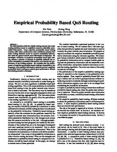
3. Region-based routing architecture The functional diagram and abstract path calculation process of our architecture is shown in Fig. 1. 3.1. Regions In our architecture, the Internet is divided into regions. We consider the Internet as a network IZ(N,L) consisting of a finite set of nodes N and a finite set of links L. Every node n2N in this network is an AS. A region RiZ(V,E) is a connected graph that is a subset of network I (Ri3I), and the union of the regions is the Internet ðI Z R1 g R2 g/g Rn Þ: One important feature of the regions is that they overlap at the borders. If Rm and Rn have an interconnecting link, then RmhRnsf. Fig. 2 gives a small representative internetwork. In this figure every node represents an AS. Fig. 3 shows a region configuration in that network. Every region consists of transit AS. Stub AS are collected into special regions called stub-regions. All links between regions appear in the topology. This is in contrast with other
Fig. 1. Functional diagram and abstract path calculation process.
I.T. Okumus et al. / Computer Communications 28 (2005) 174–188
177
Once the regions are constructed, domains inside every region exchange link states with other domains of the same region. Details of the link state exchange process are described in Section 3.2. One of the important features of our architecture is that regions do not constitute a hierarchy. There is no single agent or system that represents a region and regions do not have any intelligence. Regions are only constructed to provide boundaries for a link state exchange procedure. Fig. 2. A sample network.
approaches, which choose a representative link and ignore secondary or tertiary links. This brings richness to the topology and gives us the ability to calculate alternate paths to a destination. To construct a region we first determine the number of regions to have in the network: i. Next, we select i number of nodes in the network that has the highest degree as region leaders to construct a region. Starting from the region leader of every region, we add other nodes into the regions based on the connectivity. One rule we follow is that a node cannot be a member of more than one region, and every node is assigned to a region. Our region construction algorithm is similar to the breadth-first search for a spanning tree algorithm, but the difference is that the result is not a spanning tree, but a connected subset of the graph. Region construction process is necessary to identify the nodes in a region. After all the nodes of all the regions are identified, region numbers are assigned to the nodes. Region identifications along with node identifications are used to limit the link-state exchange in the network. Following is the algorithm we used for region construction: S is the temporary set of vertices, V is the set of highest degree nodes in the network, and R is the set of regions, and i is the number of regions. (1) Set Sn to Vn and set Rn to the graph consisting of Vn and no edges, where nZ1,2,.,i. Vn is the root of tree Rn. (2) Process vertices in Sn in order. For each vertex x in Sn add adjacent vertex y to Sn iff y is not in any Rn or Sn. (3) Replace the content of Sn with the children in Rn. Go to step 2.
Fig. 3. Regions of the sample network in Fig. 2.
3.2. Link-state exchange Inside every region, a link-state QoS routing protocol is employed. In our architecture every domain is represented by a !domainId, RegionIdO tuple. Every domain inside a region keeps a table that consists of the neighbors of the domain. We refer to this table as a peer table. In this context we define a neighboring domain as a domain that has an edge to the origin domain. Every domain inside a region keeps another table that consists of tuples !ingress domain, region IdO. We refer to this table as a peer region table. Ingress domain is a domain that has an edge to another domain in the reference region. If a domain has an edge to another domain in another region, we call this domain as an edge domain. Ingress domains are edge domains. A peer table is constructed when the routing agents are first initialized. Every domain advertises its link states to every other domain that is in its peer table. When a domain gets a linkstates message from a domain that is in the peer table, the domain accepts the link state message, updates its link-state database and forwards the message to its own peers, except the one that sent the message. This way link states of every domain reach to every other domain in that region. If a domain is not an edge domain, that domain accepts all the link-states messages and forwards them to its peers. If a domain is an edge domain, it has to carefully examine the sender, originator, and regions of the sender and the originator of the message before accepting the message and relaying it into its own region. If a message is coming from a peer that is in another region, and that domain is the originator of the message, an edge domain accepts the message, updates its database and forwards that message to its own peers that are in its own region. If a message is coming from a peer domain that is in another region, and that peer domain is forwarding the message from a domain that is not in the edge domains’ region, the edge domain simply discards the message without updating its link-state database. Domains should also be careful when forwarding link state messages. Messages are not forwarded to the sending domain. If a peer domain is in another region the message is not forwarded to that peer. When a domain gets a link state message that is from a domain in another region, the domain updates its link-state database and also updates its peer region table. This way every domain in a region constructs its peer region table that
178
I.T. Okumus et al. / Computer Communications 28 (2005) 174–188
consists of all the ingress domains of all the neighboring regions. This list of ingress domains is used for calculation of a path to a neighboring region. Our architecture tolerates inter-domain link failures. We assume that intra-domain link failures are handled by intradomain routing protocol and do not trigger an inter-domain link-state update. Whenever an inter-domain link failure occurs, this failure is automatically detected by the routing agent and this information is distributed to every other domain in the region. Also link parameters are updated periodically. If a significant change occurs in the link state, domains send out the new link states to other domains without waiting for the next update time. If an edge domain gets isolated from a region because of a link failure, other domains inside the same region use other edge domains to reach other regions. If the edge domain that is isolated is used as an ingress domain by another region, those domains in the other region use another ingress domain to that particular region. If the ingress domain is the only ingress domain to that region, regional path will be updated and there will be a path to destinations, and possibly to the subject edge domain (if it is not completely isolated from the Internet) over another region. Based on our evaluation results, especially in large networks, there are multiple ingress domains of a region and we do not expect any regional path changes. Regions can be constructed by an authority, such as ARIN [10], and domains can be assigned to a particular region based on the connectivity. One rule for region construction is that every domain inside a region should be able to find a path to every other domain in the same region without going out of the region. Region size can be determined by the authority based on the performance of the routing protocol, and region sizes need not to be fixed and we expect the region sizes will be different because of the heterogeneous connectivity of the Internet. 3.3. Path calculation process Whenever a domain accepts a new link-state message, it results in a change in the link-state database. Every domain inside region calculates a path to every other domain inside the same region. Path calculation can be on-demand or based on precalculation. When a source domain s wants to send QoS traffic to a destination domain d, s first determines the region of the destination domain (Rd). If the source domain is not in the same region as the destination domain (RssRd), the source domain calculates a regional path to the destination domain. This path consists of a sequence of regions from Rs to Rd: PRZ(Rs,.,Rd). Starting from the source domain, every ingress domain of regions on the regional path calculates a QoS path that connects the previous region to the next region on the regional path. When the source domain identifies the regional path PR, the next step is to identify an ingress domain of the next region on the regional path; then the source domain calculates
the shortest path that satisfies the QoS parameters to that ingress domain. This approach is analogous to intra-domain link-state routing approaches. In intra-domain routing, if a core router wants to transfer traffic outside its domain, the core router identifies the border router that will carry the traffic to other domains and calculates a path to that border router. After a calculation of the QoS path through its own region, the source domain sends a Path Request Message to the ingress domain of the next region. This message includes the explicit regional path and the QoS parameters. The QoS parameters embedded into the Path Request Message are not the original QoS parameters requested by the end-system. After a domain calculates a QoS path through its own region, that domain knows the QoS characteristics of that path. Let us assume the original QoS parameters were additive and values were: C1, C2, C3 and the QoS characteristics of the path calculated by the domain d1 are: c1d1!C1, c2d1!C2, and c3d3!C1. When sending a Path Request Message, d1 puts C10 ; C20 and C30 as QoS parameters where: C10 Z C1 K c1d1 ;
C20 Z C2 K c2d1 ;
C30 Z C30 K c3d1 :
The path calculation process of the source domain is repeated by every ingress domain of the regions on the regional path until the Path Request Message reaches the destination domain. The destination domain simply responds with a Path Response Message to the ingress domain that sent the message to the destination domain. Every ingress domain involved in the path calculation process relays the message back to the source domain after adding their subpaths to the explicit path object in the Path Response Message. The end-to-end QoS path is a concatenation of the subpaths calculated by ingress domains of every region on the regional path pZ ðPRs ; .; PRd Þ: When the source domain receives the positive Path Response Message, the QoS path is completely calculated and the path setup can be initiated. As it can be seen from the protocol, our goal is first to find the best QoS path inside a region, then to calculate the regional path to the destination (which consists of regions), and then to ask the ingress domain of the neighbor region to calculate a path to the next region until the path is calculated to the destination domain. The algorithm is shown in Fig. 4. We have three different sections to coordinate for this routing architecture to work: intra-region interconnections, inter-region interconnections, and stub-domains to core interconnections. 3.4. Intra-region interconnection A region consists of a number of transit AS1 (Fig. 3). A link-state flooding area of a region is broader than the region itself. We include the ingress domains of neighbor regions 1
An exception is the special regions for stub domains.
I.T. Okumus et al. / Computer Communications 28 (2005) 174–188
179
we are including stub domains in penultimate domains’ topological view by defining a region that includes only the penultimate domain and its connected stub domains. This region is called a stub region. When a path request comes to a penultimate domain for a certain stub domain, the penultimate domain simply checks the connection to that stub domain. This step is necessary to verify that the QoS metrics are in fact satisfied through the edge of the stubdomain. 3.5. Inter-region interconnection
Fig. 4. Inter-region path calculation algorithm.
in the link-state topology (Fig. 5), where an ingress domain of a region is any domain that has at least a single link to another domain in another region. Topological view of every domain in a region includes every other domain in the same region, and the ingress domains of neighbor regions. We note that although members of a region have the ingress domains of neighboring regions in their topological view, those ingress domains do not have those members in their topological view. Figs. 3 and 5 show the difference between the definition of a region and the link-state flooding area of a region. Penultimate domains—those transit domains that connect to stub domains—have an exceptional topological view. Since we are keeping stub domains out of the view of core regions for scalability purposes, and we need to calculate a path to the edge of the destination stub domain,
Having every region’s topological view include its neighbors’ ingress domains facilitates inter-region path calculation. Once a domain inside a region finds the best path through its own region to the next region, that path ends at the ingress domain of the neighbor region. The next step will be sending a Path Request Message to that ingress domain to calculate a path to a certain destination through its own region. Upon receiving the Path Request Message, if the destination domain is in its own region, an ingress domain calculates the path to the destination and sends back the result with a Path Response Message. If the destination is in another region, the ingress domain calculates a path to the ingress domain of the next region that has the available capacity, and forwards the Path Request Message to the next ingress domain with updated QoS parameters. When an ingress domain receives a Path Response Message that corresponds to a previously sent Path request Message, ingress domain appends the explicit path, which is calculated to the ingress domain that is sending the Path Response Message, to the head of the path, and forwards the Path Response Message to the originating domain of the request. With the Path Request Message, requesting routing entity will pass the updated QoS parameters and optionally the abstract regional path to the ingress domain of the next region. 3.6. Stub-domain penultimate-domain interconnection The next step is to solve the stub domain—penultimate domain interconnection issue. If we think in terms of routing, a path found by a penultimate domain to a destination and a path found by a stub domain to the same destination is the same path except that the stub domain path
Fig. 5. Link state area of regions of network in Fig. 2.
180
I.T. Okumus et al. / Computer Communications 28 (2005) 174–188
also includes the penultimate domain, because the stub domain must use the penultimate domain to transfer its traffic. In the case of multihomed networks, the same argument is valid; in that case, the choice of the penultimate domain will determine the path and the path will be the same path as the chosen penultimate domain’s path. Every stub domain has its related penultimate domain and other stub domains that are connected to the same penultimate domain in their topology. A stub domain requests a path to a destination from its penultimate domain. Once the path is calculated to the penultimate domain of the destination stub domain, one last Path Request Message is sent to the penultimate domain of the destination stub domain. The penultimate domain verifies that QoS metrics still hold to the edge of the destination stub domain. Once the path information comes back to the originating domain, QoS path is ready and path setup process is initiated using the calculated QoS path. One of the issues we need to solve is ‘how do we find the penultimate domain of a network we are trying to reach?’ Stub domains are not visible to the core of the network. This makes it hard for a domain to determine the path to that network. To solve this issue, every region can keep a nameserver that has the stub domain, penultimate AS, region information for networks. This information can be extracted from a BGP routing information base. BGP announces the whole AS path to neighbors for a destination. By looking at this message we can prepare a table that consists of a reverse tree, starting from the network, to the penultimate AS and to the region. It is important to note that we are not proposing a new QoS routing heuristic that will enable one to solve multimetric path calculation problem. There are various heuristics that can be employed in our architecture. We are providing an architecture and framework that facilitates scalable link-state routing without loss of any information due to aggregation property of hierarchical approaches. Inside every region, there can be different routing protocols running. Every region can use different heuristics to compute a QoS path with multiple metrics. As long as domain-level routing agents understand the Path Request and Path Response Messages, and be able to respond with an explicit path, our architecture works. Another important feature of our architecture is that a source domain does not have any control over the intra-domain path selection of any other domain. Intra-domain topology is completely hidden from other domains and an intra-domain path selection is responsibility of every AS. A source domain only calculates an AS level path. This will prevent malicious use of the architecture to create congestion in other domain’s intradomain links. Another important assumption we have to note is on the QoS model. As a QoS model, we are assuming that every domain allocates a certain percentage of its physical link capacity to a certain class of traffic. Bandwidth constraint model does not permit one traffic class to starve another
traffic class. A flow belonging to a certain traffic class always gets the treatment of that class as long as there is available capacity for that class to accommodate the flow. This means that at any time, there cannot be a situation where a link cannot support given traffic that has already been accepted, except for link failure cases. As we mentioned earlier, we use this architecture along with BGP. As this routing approach is used for QoS traffic, BGP is used for best effort traffic. When this routing approach stabilizes and becomes widely used over the Internet, best effort traffic can also be channeled by our routing approach and with extension to the protocol to enable it to communicate with the border routers, BGP can be completely replaced by our new routing architecture.
4. Evaluation results In this section, we explain the evaluation methodologies, test scenarios and evaluation results for our QoS routing architecture. We tested our architecture in terms of scalability. We compared our architecture with the basic approach (every domain, except stub domains, on the Internet is represented as a single entity in the topology), and analyzed the effect of the size of a region on the scalability. We also analyzed the path-finding ability of our protocol. The reason for this investigation is that our architecture uses a concatenation of regional subpaths to find an end-to-end AS-level path to a destination, and there is a possibility we will miss the best path, because the source does not have a complete view of the Internet. The best path found inside a region might not be a component of the absolute best path across the Internet. Comparison between the size of a region and the impairment of shortest path finding ability will reveal the architectures’ tradeoff between scalability and path finding ability. The question we answer is ‘how much are we sacrificing to make the architecture scalable and is the sacrifice tolerable with respect to the gain from scalability?’ 4.1. Simulation environment and topologies We evaluated our architecture using the ns2 simulation tool [11]. We constructed the topologies using the BRITE topology generator [12]. Our topologies are generated using heavy-tailed Waxman model and heavy-tailed Barabasi– Albert (BA) model [13]. We evaluated our architecture using three different topologies: 100 nodes, 1500 nodes, and 3000 nodes. All topologies consist of only transit domains. Our region structuring technique is independent of the number of AS present in the underlying network. For the topology selection, apart from topology generators, we have one other choice, which is to use topologies that are generated from BGP routing table. One source we are aware of for this kind of topologies is the data provided by University of Oregon Route Views Project [14]. One can
I.T. Okumus et al. / Computer Communications 28 (2005) 174–188
suggest that using the topologies generated from real BGP routing tables will be more realistic for the evaluation of the subject study. One important issue we have to point out with this suggestion is the possibility of the incompleteness of topologies generated by using these routing tables. Authors in [15] studied the topologies generated using Oregon Route Views BGP data and compared that with topologies they constructed using the data they collected employing several different Looking Glass sites and Internet Routing Registry. As a result of the study, authors found out that ‘there are at least about 25–50% more AS connections in the Internet than commonly-used BGP-derived AS maps reveal’. This is an important finding. Even if we generate a topology using real BGP tables, the generated topology still misses a significant amount of connectivity that exists in the Internet. The result we cited above compares two approaches, where one approach uses only one BGP table and the other one uses multiple data sources. Even the second approach has a chance to miss the existing links in the Internet. In order to evaluate the second approach’s completeness, we need to know the exact topology of the Internet, which no one has today. Whether we use topology generated by a topology generator or a topology generated using BGP data, that topology will not be the exact representation of the Internet. Main point we need to look at is whether the topology we use has the basic characteristics of the Internet topology, rather than asking whether it is a real Internet topology or not. Another point we need to carefully think is whether the topology affects the evaluation results; in other words, what is the sensitivity of the approach to the topology? Since we do not have a chance to obtain the exact topology of the Internet, and the Internet topologies generated by a BGP data misses significant amount of links that exist in the Internet, which is important to have for an inter-domain routing study, any topology we choose to use, whether it is generated by a BGP data or by a topology generator, will be missing some of the characteristics of the real Internet topology. Rather than verifying the representativeness of the topology we use in our simulations, which is out of scope of this study, we study the sensitivity of our architecture to the topology in addition to other evaluations we mentioned above. 4.2. Simulation and evaluation details We automated the region construction process using a simple heuristic. At first we determine the number of regions we want to have in the topology. Then we select the same number of nodes from the topology starting from the node that has the highest degree. We refer to these nodes as ‘region leaders’. Then following the edges of the region leaders, we add other nodes to the region. This iteration continues until all the nodes in a topology are assigned to a region. Every node in a topology is represented by a (nodeid, region-id) pair.
181
Inside each region we employed a link-state approach to distribute the topology information to every other member of the region. We only considered available bandwidth, which is advertised within the link-state, as a QoS metric in our path calculations. This bandwidth is the minimum of the inter-domain link bandwidth and the available intra-domain bandwidth to the advertised destination. We used the Bellman–Ford (BF) algorithm to select the QoS paths inside a region. The advantage of using BF is that this algorithm finds the shortest path with the requested amount of available bandwidth, which means that the paths is optimized with respect to the available bandwidthand the hop count [16]. For the calculation of an abstract regional path to a destination, we also selected the shortest regional path possible. For the simulations we ran, we used static regional paths. Once the regional path is selected, a node needs to determine an ingress node to the next region in the abstract regional path. If there is a single ingress node to next region, this selection is straightforward. If there are multiple ingress node to a neighbor region (which is highly possible), we selected the shortest path to that region that has the requested available bandwidth. As a result of these simulations, we analyzed our architecture in terms of communication, computation and storage scalability. All these measures depend on the number of regions in a topology, which determines average region size. The region sizes are not uniform. Every region has a different size depending on the selected region leader at the beginning of the region-construction process. Another important measure we considered when evaluating our architecture is whether our architecture imposes additional traffic on the Internet or not, which is also used as a measure for analysis by Apostopoulos et al. [17]. This measure is evaluated by the average number of hops in the shortest paths. If an average shortest path length (SPL) found by this architecture is longer than average of the absolute SPL of the topology, extra traffic is being imposed on the Internet by our architecture by occupying extra links. We analyzed the tradeoff between the scalability and the extra traffic by comparing the increase in the region size and the average SPL. If the average SPL is not increasing dramatically while we reduce the region size, and in turn increase the communication, computation and storage scalability, our architecture is successful. We also considered the path setup time as a measure to study our architecture. If a destination domain is in the same region as a source domain, only one path calculation takes place. If the destination domain is in another region, then path establishment time is increased based on the number of regions the destination is away. Every region should calculate the path and return the results. For the path setup time, we took the number of Path Request Messages as a measure. Every Path Request message adds to the path setup time.
182
I.T. Okumus et al. / Computer Communications 28 (2005) 174–188
4.3. 100 domain simulation Table 1 shows the simulations results for a topology with 100 nodes. For this topology we simulated our architecture using three different configurations: 1 region, 5 regions, and 11 regions. We calculated paths from each node to every other node in the topology. This means we calculated every possible path in the topology, which adds up to 9900 path calculations. All path calculation are based on a fixed-size bandwidth request. The first configuration has a single region and all the nodes are members of this region. The paths calculated on this configuration are the absolute shortest paths in this topology and we use this calculation as a basis of our comparison with other configurations. The first column in the table shows the number of regions used for the simulation. Having results for different sized regions gives us a solid foundation to evaluate our architecture in terms of the scalability measures we mentioned above. The second column in Table 1 shows the average size of a region for a given configuration. The third column shows the average length of the SPL found during the simulations; the fourth column shows the longest of the SPL found for that configuration. Column five gives the percentage of the SPL that are longer than the longest SPL of the base configuration (in this case 1 region) for a given configuration. The sixth column shows the average number of path request messages which is important for path setup time measurements. For simulation of one region, all the nodes are members of a single region and as a result the size of the region is 100. In this configuration, the number of entries in a nodes’ Forwarding Information Base is 99. Average SPL in this configuration is the average of the absolute shortest paths for this topology. We use this value as a benchmark for the other configuration results on the same topology. The longest SPL found in this configuration is 6, and since there is only one region there is no path request message for this configuration. For 5 regions, average region size is reduced by 61.4% compared to 1 region, and the average SPL is increased by 25%. For 11 regions, the region size is reduced by 81.5% and average SPL is increased by 28% compared to the 1 region configuration. This suggests a tradeoff between the scalability and the SPL. Although we are sacrificing from the average SPL, the gain from the region size is far more Table 1 Results for 100 node simulation 100 AS
Avg. region size
Avg. SPL
Longest SPL
% of longer SPL
Avg. # of PRM
1 Region 5 Regions 11 Regions
100 38.6 18.5
3.41 4.29 4.35
6 10 12
0 8.08 11.05
0 1 1.25
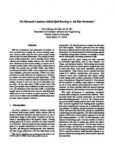
Fig. 6. SPL distribution for 100 node simulation.
than the loss from the SPL. Fig. 6 shows the SPL distribution for 100 node simulation. The average number of PRM determines the effect of our architecture on path establishment time. For 5 region configuration, there is only one PRM to calculate a path to destinations that are in another region. 11 region configuration requires 1.25 PRM on an average to calculate paths to destinations that are in other regions. To verify the results we got from the 100 node network, and to test the sensitivity of the results to the simulation topology, we decided to rerun the simulation on multiple networks with 100 nodes that are generated by the same topology generator. We generated 10 different topologies. Five of the topologies are generated using heavy-tailed BA model, and five of them are generated using heavy-tailed Waxman model. Results from these topologies show us the sensitivity of our architecture to the topology of the network. Table 2 shows the results for these simulations. As it can be seen from Figs. 7 and 8, results of all the simulations for different topologies are in parallel to the results we got for the first 100 node simulation. On all the topologies, for 5 region simulations average SPL is increased by 20–27% compared to 1 region, and for 11 region simulations average SPL is increased by 25–30% compared to 1 region average SPL. By looking at Table 2, we can observe different characteristics of the topologies. Topologies generated using BA model has significantly less Table 2 Average SPL for 10 different 100 node topologies 100 AS
1 Region
5 Region
10 Region
BA1 BA2 BA3 BA4 BA5 W6 W7 W8 W9 W10
2.93 2.92 2.99 2.92 3.08 3.4 3.37 3.4 3.32 3.37
3.65 3.55 3.68 3.51 3.75 4.31 4.05 4.22 4.11 4.20
3.75 3.73 3.80 3.66 3.85 4.37 4.26 4.34 4.35 4.39
I.T. Okumus et al. / Computer Communications 28 (2005) 174–188
Fig. 7. SPL for 10 different 100 AS topologies.
SPL than the topologies generated by Waxman model. Average region size for BA topologies is very close to the average region size for Waxman topologies. For 10 region, all BA topologies have average 20.7 domains inside a region; all Waxman topologies have 21 domains. For 5 regions, all BA topologies have 40.4 domains inside a region, and all Waxman topologies have 41 domains inside a region which are also similar to previous results. Results from the exhaustive 100 node simulation runs on different topologies suggest that results do not depend on the characteristics of a topology; our architecture performs similarly on different types of topologies. 4.4. 1500 domain simulation To analyze the performance of our approach on large networks, we simulated our approach on several different large topologies. The first one of these topologies is generated using BRITE topology generator [12] and has 1500 AS in the network. We will refer to this topology as B1500 for the rest of this section. This topology is an AS level topology as in the 100 node case and does not include any router level details of an AS. The second topology we used is generated using the same topology generator. In this case we generated 15,000 AS topology, which is
183
approximately the size of the Internet as of June 2003. To complete the simulation in a reasonable time, we extracted transit AS from the topology, and as a result we ended up with 1621 AS and 2936 interconnecting links. For the rest of this section, we will refer to this topology as B15000. We selected our third topology from University of Michigan Topology Project webpage [18] that represents the connectivity of the actual Internet on that day, which we will refer as MT1500. This topology is based on the topology generated by the Oregon Route Views data [14], and specifically from the BGP data collected on March 31, 2001. Details of how this topology is generated are described in [19]. From this topology we extracted transit AS and as a result of this reduction, our topology has 1522 AS and 6822 edges in total. For the first topology we simulated our approach using four different configurations: 10 region, 24 region, 44 region, and 60 region. For all other topologies, we only simulated our approach for one configuration and that is 60 region configuration. Table 3 shows the results for simulations using B1500 topology. For this simulation we randomly selected 1000 source–destination pairs and used the same set for path calculations on all the configurations. For these 1000 source–destination pairs, we calculated a path that satisfies a certain amount of bandwidth. Our analysis is based on the relative performance of the configurations. We used the 10-region simulation results as the base of our comparisons because of the long simulation run time of 1 region configuration on B1500 topology. In terms of average region size, 24 regions results indicate a 57.5% decrease from 10 regions simulation region size, 44 regions results indicate a 75.8% decrease relative to 10 regions, and 60 regions results indicate an 82.3% decrease. In contrast to this, 24 regions indicates a 1.4% increase in the average SPL; 44 regions indicates a 9.3% increase, and 60 regions indicates a 12.3% increase in the average SPL. Fig. 9 shows the SPL distribution for B1500 topology simulation. For the last two topologies, we used 60 region configuration, and we selected 5000 random AS pairs for the path calculation. Table 4 shows the results for these simulations and 60 region simulation results for B1500 topology simulation. Fig. 10 shows SPL distribution of 60 region configuration on B15000 topology. The average SPL on this topology for 60 region configuration is 6.21, which is comparable to 60 Table 3 Results for B1500 topology simulation
Fig. 8. Percentage changes of SPLs based on 1 region SPL being 100% for 10 different 100 AS topologies.
1500 AS
Avg. region size
Avg. SPL
Longest SPL
% of longer SPL
Avg. # of PRM
10 24 44 60
286.5 121.75 69.3 5.65
6.98 7.08 7.63 7.84
13 13 16 17
0 0 1.7 3.9
1 1.01 1.28 1.46
Regions Regions Regions Region
184
I.T. Okumus et al. / Computer Communications 28 (2005) 174–188
Fig. 10. SPL distribution for 60 region B15000 topology Fig. 9. SPL distribution for B1500 topology simulation.
region configuration of B1500 topology, which has 7.84 average SPL. The maximum SPL is the same for both the topologies and also the average number of edges are very close: 1.81 for B15000 and 2.0 for B1500. For both of these topologies, the average region size is also very close. Although we extracted transit domains among 15,000 domains in B15000 topology, the characteristics of the network is very similar to B1500 network, which is generated using the same topology generator. Results of the 60 region simulation on MT1500 topology show that the average SPL for this topology is 2.81. This average is much less than B1500 and B15000 topologies’ average SPL. Reason for this difference is high connectivity of MT1500 topology. In this topology there are 6822 edges for 1522 nodes, which means the average number of edges per domain is 4.48; in B1500 it is 2.0, and in B15000 average edges per domain is 1.81. High connectivity of the MT1500 topology also affects the average region size, because a region size also includes the ingress domains of neighbor regions. As the number of edges to other regions increases, number of ingress domains in a region’s topology also increases. On MT1500 topology simulation, the average region size is 114.7, which is more than twice the average region sizes of B1500 and B15000 topologies. If we add source and destination stub domains as two hops to the SPL of MT1500 topology, the average AS path length will be 4.81, which is less than the actual average path length visible on the Internet on March 31, 2001, which is 5.3 [20]. Although we did not calculate paths for all possible source–destination pairs, maximum visible AS path
length in our simulation is still comparable to the actual maximum visible AS length on the Internet. With consideration of source and destination stub domains, maximum visible AS path length in our architecture is 13, where in actual Internet it is 17 [20]. Although we cannot compare the results with other configurations that are on the same topology, we can compare these results with the results from the B1500 topology 60 region configuration, and B15000 topology 60 region configuration. Results from MT1500 topology show that our architecture performs significantly better in terms of average SPL in highly connected networks. The SPL distribution for this simulation is shown in Fig. 11. Figs. 12 and 13 show the relative percentage changes of average SPL and average region size for 100 nodes and B1500 topology simulations, respectively. Fig. 14 shows the percentage changes on the SPL and region size for 10 different 100 domain topologies. As it can be seen from the figures, gain from the region size is always far more than the increase in the SPL. Throughout our simulations we used bandwidth as the QoS metric. It is shown in [21] that deciding a simple path which satisfies multiple additive metric constraints or multiple multiplicative metric constraints is NP-complete. This limitation lead researchers to develop heuristics [22] and metric selection criterias [21] to solve multi-metric path
Table 4 Results for 1500 node 60 region simulations 1500 AS
Avg. region size
Avg. SPL
Longest SPL
Number AS
Number of links
B1500 B15000 MT1500
50.65 50.3 1116.4
7.84 6.21 2.81
17 17 11
1500 1621 1522
3000 2936 6822 Fig. 11. SPL distribution for 60 region MT1500 topology.
I.T. Okumus et al. / Computer Communications 28 (2005) 174–188
185
Fig. 12. The average SPL and the average region size comparison for 100 node simulations.
Fig. 14. SPL and region size percentage changes for 10 different 100 domain topologies.
computation problem. It is also shown in [21] that bandwidth and delay are not independent metrics. These are the reasons for us to consider only the available bandwidth as a QoS metric and any of the developed heuristics can be used in our architecture. Results of 1500 nodes simulations support the results of 100 nodes simulations. For 1500 nodes, percentage change in the average SPL with decreasing region size is far less than the percentage change in 100 nodes simulations. This indicates that our architecture performs better in bigger topologies. There is a clear tradeoff between the region size (which effects the communication, computation and storage scalability) and the average SPL. As the topology gets larger, scalability becomes much more important and our results suggest that the increase in the SPL is far less than the gain from the scalability. Region-based routing can have economical effects on the Internet. Although we are not analyzing the economic effects, from the findings of our simulations we can comment on the economic effect of our architecture. As we show in Table 3, as we change the size of a region in a network, the average SPL in the network for that particular region configuration increases. If we take that every link has
a unit economic cost, then shortest length path becomes shortest cost path and when the number of regions increases, average cost of the path also increases. This is the tradeoff of our architecture. 4.5. 3000 domain simulation Last simulation result is shown in Table 5. This simulation is performed on a 3000 node topology. We used only one configuration on this topology, which has 128 regions. The reason for us to perform this simulation is to demonstrate that our architecture can work on a huge network. Currently there are approximately 7.6 stub-AS on the Internet for every one transit-AS. Because of this 3000 AS network corresponds to around 23,000 AS Internet.
5. Related work In this section, we review various inter-domain routing approaches. These approaches can be classified as pathvector approaches, hybrid approaches (link-state and pathvector together), and hierarchical approaches that are proposed to make the link-state-based approaches scalable. Currently, a majority of the Internet uses BGP4 [3] for inter-domain routing. This protocol is based on a path vector algorithm. Every AS that uses BGP advertises to its BGP peers the reachibility information for its domain. There are several studies about the problems BGP is facing in today’s Internet [23–26]. Major concerns with BGP are the convergence time and the size of the BGP routing table. Implicit inter-domain traffic engineering using BGP also Table 5 Results for 3000 node simulation
Fig. 13. The average SPL and the average region size comparison for B1500 node simulations.
3000 AS
Avg. region size
Avg. SPL
Longest SPL
Max. number of PRM
128 Regions
47.7
9.18
20
2
186
I.T. Okumus et al. / Computer Communications 28 (2005) 174–188
adds stress to these concerns. There are attempts to add QoS capability to BGP [27–29], but the proposed solutions make BGP even more complex. The most common approach to solve the scalability problem of link-state-based inter-domain routing is to use a hierarchy [4,6]. Hierarchical approaches are known to be lossy in terms of domain level information, since several domains have to be represented as if they are a single domain, and all the parameters concerning the inter-domain routing have to be aggregated into a single set of parameters. As a result of this, a routing algorithm may not be able to find a path to a destination that satisfies certain requirements, even though one exists. Alaettinoglu and Shankar [2] propose to use viewservers to solve the problems of hierarchical routing. This approach basically uses subsets of the Internet topology to calculate a path to a destination by merging views of the viewservers that exist in the topology in a hierarchical manner. Viewservers provide topological information on their level of the hierarchy. One concern with this approach is that the size of the merged view at the source can increase computational and storage costs. Another drawback is that path setup time is increased by the number of requests for views from the viewservers. An approach that addresses the inter-domain QoS routing problem is described in [7]. This approach also uses hierarchies to make the approach scalable. When constructing the hierarchical groups of domains, all the gateways are included in a graph. Evaluation results of this routing approach are not available, making it difficult to analyze this approach. Estrin et al. [5] present a hybrid approach to solve the inter-domain routing problem. This approach proposes to use the path-vector approach for most common Type of Service (ToS) and policy constraints, and the link-state approach for rare ToS and policy constraints. This proposal does not address the scalability of the link-state part of the proposed architecture. In [6] Streenstrup proposes using link state approach to implement inter-domain policy routing with source specified route generation. This gives a domain the ability to distribute the route information to the domains it chooses and to calculate the route to a specific destination based on its own reasoning. This approach proposes the use of superdomains, which are collections of multiple domains into a representative single domain that are built in a hierarchical way to make the approach more scalable. The problem with superdomains is the loss of information during the abstraction process. Zhang and Kantola [30] focuses on how QoS routing can be realized and used to setup end-to-end QoS paths in a Diffserv network. It can be seen from this work that the main bottleneck is the lack of knowledge on whether the resources are available beyond an AS or not and that lack of knowledge tends to increase the path setup time. There is a survey paper by Chen and Nahrstedt [8], which analyzes
the QoS routing approaches with their advantages and disadvantages. This paper helps to understand the issues involved in QoS routing problem. An example work for bypassing BGP for resiliency purposes is ‘Resilient Overlay Networks (RON)’ by Andersen et al. [31,32]. This work aims to provide more robust and resilient operation for applications over the Internet. End points called RON nodes configure themselves into an overlay network. Connections among participating RONs are calculated based on link parameters between two RONs. The end RONs calculate the best path to another RON using the overlay topology. Source routing is achieved by IP encapsulation. The goal of this work is not to provide QoS, but rather to make the overlay network resilient and more efficient and immune to the faults of the network caused by BGP. Another work on ‘End-to-End Effects of Internet Path Selection’ by Savage et al. [33] analyzes the paths taken in the Internet and tries to show that in most cases there are better alternate paths than the one given by current routing protocols. This work shows that in 30–80% of the cases, there is an alternate path with significantly superior quality. These last two work support our idea of forwarding our QoS traffic on a path that we select using the link metrics independent of the route provided by traditional interdomain routing protocol (such as BGP). We do not want to change the infrastructure of the Internet. Our solution sits on top of the current topology and QoS traffic is forwarded using QoS paths calculated by our approach and best effort traffic is forwarded along the paths that are advertised by the current routing protocols.
6. Comparison of results with the viewserver approach To evaluate the performance of our architecture, we need to compare it with another system. One study that has a methodology to evaluate the routing approach and has the results that has properties with which we can compare our architecture is Alaettinoglu and Shankar [2]. In this work performance of the routing approach is studied in terms of scalability and path calculation ability. Although results from this study depend on the underlying network topology, size of the topology used for this study is comparable to the size of the topology we used for 1500 node simulation. The topology used by Alaettinoglu and Shankar [2] has 11,100 nodes which includes 1000 Metropolitan Area Networks, 100 regional networks, and 10 backbones. If we exclude stub domains from this topology, there are 1110 transit networks in the topology. In our topology, we have 1500 transit nodes in the topology. To calculate the complete path, a source queries multiple viewservers, merges these views at the source and then calculates the path. If the source cannot find a path in the merged view, the source queries more viewservers to enrich
I.T. Okumus et al. / Computer Communications 28 (2005) 174–188
the merged view. To measure storage scalability, authors used size of the topology kept at each source, and merged view size. These measures give the memory requirement at each source. Another measure used by the authors is the number of query messages to calculate a path to a destination, which in turn determines the path calculation time. We will compare these measures with results of our architecture. For the storage scalability, our measure is the average region size. For path calculation time, as we mentioned earlier, we use average number of PRM. Authors of [2] used different configurations to evaluate the effect of each configuration to the results. Since authors suggested that vertex-ex scheme is the best configuration, we will use results from this configuration to compare our results. For storage scalability, we will compare our results with merged view size results of [2], because that gives the information about the required amount of storage to calculate a path. In [2], average merged view size for vertex-extension configuration is 362.15, and average number of viewservers queried to obtained the merged view size is 7.51. In our architecture, for 1500 node topology, average region size is 286.5 for 10 region, 121.75 for 24 region, 69.3 for 44 region, and 50.65 for 60 region configuration. Average number of PRM are 1 for 10 region, 1.01 for 24 region, 1.28 for 44 region, and 1.46 for 60 region configurations. In our configurations, worst case for storage scalability is 10 region configuration, which has 286.5 average region size. Although this is the worst case in our architecture for this topology, average region size is less than the merged view size. In terms of the path calculation time, worst case in our architecture for this topology is 60 region case, which requires on average 1.46 PRM to get the complete path to a destination. This is much less than 7.51 view query messages to get a merged view to be able to calculate a path to a destination in viewserver architecture. If we consider all the configuration cases for viewserver hierarchy, average merged view size ranges from 71.03 to 396.8. In our architecture, average region sizes ranges from 50.65 to 286.5. Although these are not the only possible configurations for our architecture, results are still better than viewserver results. Comparison results are listed in Table 6. Table 6 Comparison of region-based approach with viewserver approach
Region-based
Viewserver
Number of nodes
Region size
Number of messages
1500
50.65/286.5
1/1.46
Number of nodes
Merged view size
Number of messages
1100
23/362.15/486
3/7.51/8
187
7. Conclusion In this paper we introduced a novel scalable link-state based source-specified inter-domain QoS routing architecture. Our architecture represents every AS as a single routing agent in the Internet topology. These routing agents are divided into non-hierarchical regions. Edge-to-edge ASlevel QoS paths are calculated as concatenation of sub-paths that are calculated by ingress domains of the regions along the regional path. The performance of the architecture is evaluated with simulations. Results of analysis show that this approach’s scalability depends on the size of a region. Further analysis shows that as the scalability of the approach increases, the average path length is also increased, but the gain from the scalability is far more than the loss from the increase in the average path length, especially with large topologies. We also observed that results do not depend on the topology used in the simulation, and architecture gives similar results on different topologies that have different characteristics. The architecture provides the following advantages: † † † †
Reduced link-state advertisement messages. Limited link-state flooding area. Reduced topology table size in each routing agent. Reduced forwarding table size.
These items correspond to the architecture’s communication, computation, and storage scalability. To the best of our knowledge, our architecture and the resulting scalability solutions are novel.
References [1] Asia Pacific Network Information Center, http://www.apnic.net/ mailing-lists/bgp-stats/index.shtml [2] C. Alaettinoglu, A.U. Shankar, The viewserver hierarchy for interdomain routing: protocols and evaluation, IEEE Journal on Selected Areas in Communications 13 (8) (October 1995) 1396–1410. [3] Y. Rekhter, T. Li, A border gateway protocol 4 (bgp-4), RFC1771, March 1995. [4] Y. Rekhter, Inter-domain routing protocol (idrp), Internetworking: Research and Experience 4 (1993). [5] D. Estrin, Y. Rekhter, S. Hotz, Scalable interdomain routing architecture, Proceedings of ACM SIGCOMM’92 Applications, Technologies, Architecture, and Protocols for Computer Communication, Baltimore, Maryland, USA, August 1992. [6] M. Streenstrup, An architecture for inter-domain policy routing, RFC 1478, June 1993. [7] S.-H. Kim, K. Lim, C. Kim, A scalable qos-based inter-domain routing scheme in a high speed wide area network, Computer Communications 21 (4) (February 1998) 390–399. [8] S. Chen, K. Nahrstedt, An overview of quality-of-service routing for the next generation high-speed networks: Problems and solutions, IEEE Network, Special Issue on Transmission and Distribution of Digital Video, 1998.
188
I.T. Okumus et al. / Computer Communications 28 (2005) 174–188
[9] K. Nichols, B. Carpenter, Definition of differentiated services per domain behaviors and rules for their specification, RFC 3086, April 2001. [10] American registry for internet numbers, http://www.arin.net/ [11] The network simulator-ns-2, http://www.isi.edu/nsnam/ns/ [12] Boston university representative internet topology generator (brite), http://www.cs.bu.edu/brite/ [13] A. Medina, A. Lakhina, I. Matta, J. Byers, Brite: an approach to universal topology generation, in: Proceedings of the International Workshop on Modeling, Analysis and Simulation of Computer and Telecommunications Systems—MASCOTS ’01, Cincinatti, OH, 2001. [14] D. Meyer, University of Oregon route views project, http://www. routeviews.org/ [15] H. Chang, R. Govindan, S. Jamin, S. Shenker, W. Willinger, Towards capturing representative as-level internet topologies, Computer Networks Journal 44 (6) (2004). [16] R.A. Gue´rin, A. Orda, D. Williams, Qos routing mechanisms and ospf extensions, IEEE Global Communications Conference 1996, 1996. [17] R. Guerin, A. Orda, Computing shortest path for any number of hops, IEEE/ACM Transactions on Networking 10 (5) (October 2002) x. [18] Topology Project, http://topology.eecs.umich.edu/ [19] Q. Chen, H. Chang, R. Govindan, S. Jamin, S. Shenker, W. Willinger, The origin of power laws in internet topologies revisited, IEEE of the 21st Annual Joint Conference of the IEEE Computer and Communications Societies, Infocom 2002, New York, NY, June 2002. [20] Asia pacific network information center, routing table report, http:// www.apnic.net/mailing-lists/bgp-stats.archive/2001/03/msg00030. html [21] Z. Wang, J. Crowcroft, Quality-of-service routing for supporting multimedia applications, IEEE Journal of Selected Areas in Communications 14 (7) (September 1996) 1228–1234. [22] T. Korkmaz, M. Krunz, Multi-constrained optimal path selection, in: Proceedings of the 20th Annual Joint Conference of the IEEE Computer and Communications Societies April 2001; 834–843.
[23] G. Huston, Commentary on inter-domain routing in the internet, RFC 3221, December 2001. [24] K. Varadhan, R. Govindan, D. Estrin, Persistent route oscillations in inter-domain routing, Computer Networks 32 (1) (1999) 1–16. [25] D. Obradovic, Real-time model and convergence time of bgp, Infocom 2002, The 21st Annual Joint Conference of the IEEE Computer and Communications and Societies, June 2002. [26] T.G. Griffin, G. Wilfong, An analysis of bgp convergence properties, ACM SIGCOMM’99 Applications, Technologies, Architectures, and Protocols for Computer Communication, August 1999. [27] B. Abarbanel, S. Venkatachalam, Bgp-4 support for traffic engineering, Internet draft, work in progress, September 2000. [28] C. Jacquenet, Providing quality of service indication by the bgp-4 protocol: the qos-nlri attribute, Internet Draft, work in progress, June 2003. [29] J. Hwang, J. Altmann, H. Oliver, A. Suarez, Enabling dynamic market-managed qos interconnection in the next generation internet by a modified bgp mechanism, The IEEE International Conference on Communications, New York, New York, USA April 2002;. [30] P. Zhang, R. Kantola, Mechanisms for inter-domain qos routing in differentiated service networks, First International Workshop on Quality of Future Internet Services (QofIS’2000), September 2000. [31] D.G. Andersen, H. Balakrishnan, M.F. Kaashoek, R. Morris, The case for resilient overlay networks, Proceedings of the Eighth Workshop on Hot Topics in Operating Systems HotOSVIII, May 2001. [32] D. Andersen, H. Balakrishnan, F. Kaashoek, R. Morris, Resilient overlay networks, Proceedings of the 18th ACM Symposium on Operating Systems Principles, October 21–24, 2001. [33] S. Savage, A. Collins, E. Hoffman, J. Snell, T. Anderson, End-to-end effects of internet path selection, Proceedings of ACM SIGCOMM’99 Applications, Technologies, Architecture, and Protocols for Computer Communication, September 1999.