SciPost Physics
Submission
Interacting quantum walk on a graph Alberto D. Verga1* 1 Aix-Marseille Université, CPT, Campus de Luminy, case 907, 13288 Marseille, France *
[email protected]
arXiv:1805.02929v1 [quant-ph] 8 May 2018
May 9, 2018
Abstract We introduce an elementary quantum system consisting of a set of spins on a graph and a particle hoping between its nodes. The quantum state is build sequentially, applying a unitary transformation that couples neighboring spins and, at a node, the local spin with the particle. We observe the relaxation of the system towards a stationary paramagnetic or ferromagnetic state, and demonstrate that it is related to eigenvectors thermalization and random matrix statistics. The relation between these macroscopic properties and interaction generated entanglement is discussed.
Contents 1 Introduction
1
2 Model
2
3 Phenomenology
5
4 Spectrum
8
5 Discussion and conclusion
11
A Python codes
13
References
16
1
Introduction
An isolated system, initially out of equilibrium, relaxes to thermal equilibrium. The physical mechanisms behind this elementary experimental fact range from thermodynamics to the fundamentals of quantum statistical physics. Indeed, the very existence of a relaxation seems to be in contradiction to the unitary evolution of physical systems. Already in the twenties von Neumann [1] realized that despite the global conservation of the entropy, expected values of local observables 1
SciPost Physics
Submission
approached their microcanonical values for most quantum states [2,3]. The aim of von Neumann was to demonstrate ergodicity in quantum systems without the assumption of disorder, the Boltzmann Stoßzahlansatz used in his H-theorem. In the way, von Neumann assumed that macrostates must possess an enough rich structure, which now we can relate to quantum chaos [4]. In the same spirit Landau and Lifshitz stated that averaging over a Gibbs distribution is essentially equivalent to taking the expected value of an observable in a given energy state [5, 6]. In the recent literature, hypothesis of this kind are known as the “eigenvalue thermalization” [7–11]: Deutsch [7] assumed an integrable system perturbed by a random matrix Hamiltonian, assumption that ensures Gaussian eigenstates and the validity of large deviations estimates for the fluctuations around the microcanonical values of the observables; Srednicki [8] showed that thermalization follows from the Berry’s conjecture of chaotic eigenstates [12], stating that in a semiclassical approximation of a classically stochastic motion, the corresponding wavefunction becomes a Gaussian random function. The eigenvalue thermalization hypothesis could be experimentally tested using an optical lattice of interacting bosons [13]. Therefore, in order to explain the relaxation of an isolated system, in a pure quantum state with a well defined energy, one must identify the basic mechanisms leading to thermal, or better, chaotic energy eigenstates. It is worth mentioning Cardy’s view that thermalization occurs in a pure state as a consequence of interference and entanglement with no need of ergodicity or coupling to a heat bath [14]. In this paper we investigate what are the ingredients needed for a quantum isolated system to reach a highly entangled state amenable to thermal behavior. At variance with the usual approach in which one defines the quantum system by a Hamiltonian and solves the Schrödinger equation to obtain the energy levels and states, we are more interested in the mechanisms leading to “typical” quantum states; we want to explore the possibility of constructing such states from a series of local unitary operations applied to an initially particular state, which builds to a generic one possessing the properties of a thermal state. Accordingly, we adopt a quantum information approach in which the quantum state is viewed as a resource that can be manipulated by a series of one or two qubits gates [15,16]. As a consequence of the tensor product structure of the many-body quantum state, a network or graph of nodes and edges constitutes a natural representation of the physical system. Consequently, we will consider a system defined on a graph upon which unitary operations essentially result in shuffling and swapping state amplitudes. The model is presented in the next section, followed by a brief account of the phenomenology and a characterization of the observables; we find that the subsystems set in a stationary state with well defined physical properties. In addition, we compute the spectrum of the unitary operator by exact diagonalization to get full information on the structure of the eigenvectors and the statistical distribution of the eigenvalues. Finally, we discuss the role of degeneracy and entanglement in thermalization.
2
Model
In this work we propose quantum systems defined on a network (a graph of nodes and links), with two kinds of degrees of freedom: an itinerant one, we call a particle (or walker) that can jump between neighboring nodes, and fixed ones, attached to each nodes, we call spins (or qubits). The “space” is specified by the topology of the graph; “time” is counted in steps, where the unitary transformation of the previous state is applied. The “evolution” of this state is given by the rules governing the particle jumps between the network nodes, its interaction with the graph spins, and
2
SciPost Physics
Submission
2 0
1
4 0
2
3
2
1 0
0
1
0 0
1
Figure 1: Graph definition. Each node is labeled by an integer x (in black), which corresponds to the spin location and particle position. The subnodes of node x are labeled by c (in red) in increasing order of the neighbors y of x, they correspond to the particle interanal degree of freedom (color). the interactions between spins. The model can be viewed from the point of view of quantum information, and in particular, the so-called one-way quantum computer, in which a highly entangled cluster state is the resource on which a measurement protocol drives the computation [17]. We replaced the projective operation (measure) on the cluster state (a set of interacting qubits) with the interaction of the graph state with a quantum walker [18]. More formally, we consider a set of N half spins that defines the nodes x of a graph G; each spin s x interacts with a finite number of other spins s y , determining the graph connectivity. Two interacting spins belong to the same graph edge (x, y). A particle can jump between nodes, along the connected edges, according to its internal degrees of freedom c, we call colors (see Fig. 1). The particle interacts with the node spin it visits. The Hilbert space of the quantum system is spanned by the basis vectors |x cs〉, where x = 0, . . . , N − 1 label the nodes (particle position), c = 0, . . . , d − 1 the particle color with d the maximum graph degree, and s = s0 s1 . . . sN −1 is a set of N binary numbers s x = 0, 1, specifying the two values of the spin, ‘0’ up, ‘1’ down. The Hilbert’s space dimension is then N × d × 2N . We use throughout ħ h = 1. The spin-spin interaction changes the phase of the ‘11’ two spins configuration, CZ |x cs〉 = |x cs〉 − 2s x s y |x cs〉
(1)
where (x, y) are the edges converging at x; if restricted to a two spins space its matrix form would be diag (1, 1, 1, −1). An important property of the CZ gate is that it maximally entangles two x oriented spins (both in one of the eigenstates |±〉 =
|0〉 ± |1〉 p 2
3
SciPost Physics
Submission
Table 1: Graphs. First row, three variants of a regular 8 vertex graph; second row, a symmetric chain ‘X’ and two random graphs, R(3, 12) with regular 3 degrees per node, and G(12, 3) with also 12 nodes, and mean degree of 3. 3 2 6
0
7
0
1
6
6 1 3
5
2
4
cube ‘c’
2
4 0
3
0
11
11
6
7
9 6
1 7
8
2
10
random ‘R’
3
2
8
3
5
5
möbius ‘m’
5 4
chain ‘X’
4
5
4
ladder ‘l’
1
7
7
1 0
2
3
1 6
8
7 9
4
10 5
0
random ‘G’
of the Pauli matrix σ x ). The spin-particle interaction, SW |x, 0, s0 . . . s x = 1 . . .〉 = |x, 1, s0 . . . 0 . . .〉 ,
(2)
SW |x, 1, s0 . . . s x = 0 . . .〉 = |x, 0, s0 . . . 1 . . .〉 .
(3)
exchange the ‘0, 1’ colors with the ‘1, 0’ local spin, respectively; hence it can flip individual spins; restricted to a two qubit space it is the usual swap gate. In addition to these local interactions, the particle executes a quantum walk by swapping its position x with the neighboring nodes y, controlled by the different colors, one for each of the d edges; the motion operator MV is defined by, MV |x c y s〉 = | y c x s〉 , (4) where c x , c y are the corresponding colors. Finally, the particle color at node x changes at each step of the walk, by application of the coin CO = GR, 2 0 0 0 〈x c s | GR |x cs〉 = − δc,c 0 δ x,x 0 δs,s0 , (5) dx the grover coin, or CO = FT the fourier coin: 1 〈x 0 c 0 s0 | FT |x cs〉 = p exp(i2πcc 0 /d x ) δ x,x 0 δs,s0 ; dx
(6)
where d x is the degree of node x. The grover coin distributes the amplitudes equally between the starring edges of a given node, thus respecting the graph geometry, while the fourier operator is an unbiased coin that equally superposes the amplitudes over the edges (much as a classical coin 4
SciPost Physics
Submission
in a random walk). In two dimensions the grover matrix reduces to σ x , and the fourier matrix is the Hadamard matrix. The evolution of the system is ensured by the repeated application of the unitary operator U: |ψ(t + 1)〉 = U |ψ(t)〉 ,
U = CZ SW MV CO ,
(7)
(we use 1 as the time unit) where GR acts on colors, MV on nodes and colors, SW on colors and spins, and CZ between spins. In Appendix A we present the numerical implementation of the model. Typical graphs are represented in Table 1. It is worth remarking that the model thus described do not contain dimensional parameters, nor adjustable parameters: its structure is determined by the graph and its dynamics by U, which is a pure numerical matrix. In addition, no obvious symmetries are present, due in particular to the subnode labeling that controls the motion of the particle, which depends on the arbitrarily denoted nodes. More importantly, although U is defined by strictly local rules, its corresponding effective Hamiltonian, H ≡ i ln U ,
(8)
is, in general, nonlocal, and hence do not have an immediate physical significance.
3
Phenomenology
In order to investigate the properties of the quantum state |ψ(t)〉, build after t applications of the unitary matrix U, we define macroscopic quantities characterizing the probability distribution of the particle over the nodes p(x, t) (density), and the mean value of the spin s(x, t) in the z direction (graph magnetization): p(x, t) = Trcs ρ(x cs; t) ,
s(x, t) = Tr y c σz (x)ρ( y cs; t) ,
where ρ = ρ(x cs; t) = |ψ(t)〉 〈ψ(t)| ,
|ψ(t)〉 =
X
ψ x cs (t) |x cs〉
(9)
(10)
{x,c,s}
is the density matrix at step t of the total system, ψ x cs are complex amplitudes, and Trl is the partial trace over the degrees of freedom corresponding to the label l = x, c, s; σz (x) is the z-Pauli matrix of node x. The mean value of the spin density over time is, s(t) =
T X 1 s(x, t) T − t 0 + 1 t=t
(11)
0
where t 0 is a suitable initial time in the stationary state, chosen to avoid the transitory relaxation. In addition to these local properties, we can characterize global properties of the system’s state, using the entanglement von Neumann entropy; we split the total degrees of freedom into two sets, one among position, color and spin l = x, c, s, and the other including their complementary set ¯l = {c, s}, {x, s}, {x, c}: ENTl(t) = − Tr ρ(l; t) log ρ(l; t) ,
5
ρ(l; t) = Tr¯l ρ
(12)
SciPost Physics
Submission
Table 2: Lattice graphs: comparison of the cube and möbius graphs using both coin operators. Row 1, position distribution over the 8 nodes; Row 2, spin distribution; Row 3, mean spin as a function of step number; Row 4, entanglement entropy l = x, c, s. The images show the initial and final 40 steps. 2
3
0
7
7 0
1
6
6 1 3 2
4
5
4
Grover
Fourier
Grover
1
40
360
400
0
t=0
40
360
400
1
t=0
t=0
360
360
400
1.0
s = 0.02
0.8
0.6
0.6
0
100
200
step t
300
1
40
360
400
t=0
1.0
0.4
360
1.0
s = 0.10
0.8
0.6
0.6
0.4
100
200
step t
300
0.4
0
100
200
step t
300
0.0
400
4
3
3
's' = 3.5 'x' = 2.0 'c' = 1.6
1 0
0
100
200
time
300
400
2 's' = 3.5 'x' = 2.0 'c' = 1.6
1 0
0
100
200
time
300
2
0
400
's' = 4.4 'x' = 3.0 'c' = 1.6
1 0
100
200
time
300
400
ENTl(t)
4
3
ENTl(t)
4
3
ENTl(t)
4
2
s = − 0.00
0.2
0.0
400
1
400
0.8
0.2 0
40 0
1
400
0 1
40
360
s = − 0.00
0.0
400
t=0
0
0.2
0.0
0
1
1
t=0
400
0.8
0.2
ENTl(t)
40
s(t)
1
0.4
t=0
0
s(t)
s(t)
1.0
0
40
0
400
1
1
40
360
Fourier
1
s(t)
t=0
5
0
100
200
step t
300
400
2 's' = 4.5 'x' = 3.0 'c' = 1.6
1 0
0
100
200
time
300
400
where we adopt the notation log = log2 for the logarithm in base 2, and ρ(l; t) is the partial trace over the complement ¯l of the label l, of the pure state density matrix. We present in Table 2 an overview of the properties of the interacting quantum walk for two similar graphs (same number of nodes and same regular degree), the ‘cube’ and ‘möbius’, and two choices of the coin operator GR, and FT. The image of the probability to find the walker at node x shows an interesting difference between the two graphs (first row). The walker on ‘c’ is splitted into two states, one on the nodes ‘0257’, and the other on ‘1346’, which are path with distance 2 steps (according to the node numbering). These two states are related by a swap symmetry, wich is precisely the action of the MV operator on the position subspace. Such alternating pattern is not possible on the ‘m’ graph, which presents a uniform distribution of the position. The graph magnetization tends to be uniform (second row), and generally sets in a ‘paramagnetic’ state (with vanishing mean spin), unless for ‘m’ with the grover coin. The combined action of SW and CZ is to flip and entangle spins, which happens when node spins are in a superposition of zero total spin. In the case of the ‘m’ graph, with the grover coin that respects the graph symmetry, some frustration 6
SciPost Physics
Submission
3
2
4
1
ENTl(t)
0 8
6
0.5 0.0
7 0 2 4 6 8 20
0 2 4 6 8 20
'c' 'x' 's'
1.0
5
0
10
20
30
40
time
50
60
70
80
1.0 0.5 30
40
50
60
70
80
0.0
1 0 30
40
50
60
70
80
1
Figure 2: Cycle graph with 9 vertices. Entanglement entropy as a function of time step, l = x, c, s (top panel); position distribution probability (middle panel), and magnetization (bottom panel). appears due to the existence of cycles with an odd number of nodes; this feature is absent in the ‘c’ graph. The fourier coin breaks the distinction between cycles by superposing the amplitudes around each node, and then it can avoid this kind of frustration. In this respect, the behavior of the entanglement entropy is illuminating. The coin entropy is maximal, whatever the coin; we can thus concentrate on the position and spin entropies. The position and spin entanglement entropies differ, between ‘c’ and ‘m’, in just one qubit: while the ‘cube’ encode two qubits into its position (corresponding to a subset of 4 nodes), the ‘möbius’ graph encodes three qubits, the maximum possible for 8 nodes. This behavior can be related to the cycles of four nodes observed in the ‘cube’, not present in the ‘möbius’ graph. The stationary values of the entropy are independent of the type of coin used in the quantum walk. The scenario just presented is substantiated by the behavior of similar graphs with a higher number of nodes. We considered ladders with even and odd number of rungs, periodic ladders like ‘c’ (planar graphs), or antiperiodic like ‘m’ (graphs with one crossing). Even ladder graphs show the same magnetization and entanglement properties as ‘c’; odd ones (for example, a five node length ladder, forming two pentagons), exchange their entanglement properties: the planar graph can code a supplementary qubit with respect to the crossed one. Crossed graphs, independently of the number of ladder rungs, support a non vanishing magnetization (with the grover coin). More generally, random graphs with the same number of nodes and similar regular or mean degree, behave like the ‘möbius’ or larger equivalent graphs, suggesting that it is the “typical” case: the ‘cube’ class, is special in the sense that the position entanglement entropy do not reach its maximum value, reflecting the existence of cycles symmetrical by swaps. To better appreciate the interplay of the interaction operators SW and CZ, we present the dynamics of a cyclic graph (with 9 nodes) in Fig. 2. The initial state is a superposition of spin up and down at node 0: |000 + |001〉〉 |ψ(0)〉 = , p 2 7
SciPost Physics
Submission
0.8
s¯
0.6 0.4 0.2 0.0
0
2
4
6
N
8
10
12
Figure 3: Complete graph of order N magnetization. (a basis ket is, for this graph, an eigenvector of U). After an initial cycle, the entanglement entropy start to get values of 1 for the three types of degrees of freedom l = x, c, s; in particular, after about 50 steps, a spin qubit is present. This is related to the appearance of a pair of neighboring zero spin nodes (white squares), the CZ entangles. The position entanglement entropy also codes one qubit, which can be related to the two correlated nodes (red squares), appearing for the first time at step 24. Note that entanglement arise just after the completion of a cycle: this is an effect of the swap motion that allows superposition of amplitudes only after a turn (that may depend on it parity, for a given subnode labelling). We also note that there is no straightforward relationship between entanglement and magnetization: the mean value of the spins over all nodes, mixes independent and correlated spins. However, we observed that magnetization growth with the degree of the graphs, in the case of the grover coin. For a given number of nodes, the increase in the number of edges is generally accompanied with an increase of the magnetization. For the complete graphs, larger ones show larger magnetization. This fact is well illustrated by the case of complete graphs K(N ), as shown in Fig. 3, where the magnetization is represented as a function of the number of nodes N . In contrast, for the fourier coin the magnetization generally vanishes, strengthening the fact that the value of the asymptotic magnetization is not directly determined by the graph geometry or its entanglement properties.
4
Spectrum
To get some insight into these phenomenological observations it is interesting to relate them with the spectrum of U. Using exact diagonalization, we solve the eigenvalues equation, U |n〉 = e−iEn |n〉
(13)
to find En , the quasienergies in the band En ∈ [−π, π], and their corresponding eigenstates |n〉. We denote vn the complex eigenvector coordinates of level n in the |x cs〉 representation: vn (x cs) = 〈x cs|n〉 . We define a Shannon entropy using pn = |vn |2 as the probability distribution. The Shannon entropy SHA, X SHA(n) = − |vn (x cs)|2 log |vn (x cs)|2 (14) x cs
8
SciPost Physics
Submission
Table 3: Spectrum. Columns: 1) graph; 2) quasienergy histogram; 3) spacing distribution compared to the Gaussian unitary ensemble or Poisson distribution (solid line); Shannon entropy. Rows: 1) cube, 2) möbius, 3) chain, and 4) random graph G = G(8, 3) with FT coin. Graph
Quasienergy
Spacings
0.5
0
7
1
6
0.8
0.4 0.3
p(s)
P(En )
2
3
0.2 0.0 1.0
5
0.5
0.0
En /π
0.5
6 3
0.2 0.0 1.0
2 4
0.3
5
0.5
0.0
En /π
0.5
4 7
0.2 0.0 1.0
8
0.0
En /π
0.5
1
6
3 7
0 5
0.5
1.5
2.0
2.5
3.0
2
3
4
5
6
1.0
1.5
2.0
2.5
3.0
level spacings s
0.6 0.4
1
level spacings s
1.0 0.8
0.4 0.3 0.2
0.6 0.4 0.2
0.1 0.0 1.0
1.0
0.4
0.0 0
1.0
p(s)
P(En )
4
3.0
0.2
0.5
0.5 2
2.5
0.8
0.4
5 6
2.0
1.0
p(s)
3
P(En )
0
1
1.5
0.6
0.00.0
1.0
0.6 2
1.0
level spacings s
0.2
0.1
1
0.5
0.8
0.4
p(s)
P(En )
7
0.4
0.00.0
1.0
0.5
0
0.6
0.2
0.1
4
Shannon
0.5
0.0
En /π
0.5
1.0
0.00.0
0.5
level spacings s
is a measure of the deviation of pn to the uniform distribution, and hence it also quantifies the ‘localization’ of the vn eigenvectors in Hilbert space (not specifically localization is space –which is not a relevant concept for the graph); we will consider as “typical” an eigenvector whose Shannon entropy is about its maximum. Our system lacks a conserved local Hamiltonian from which we could define a typical energy, or associate an energy to the initial state; it is then convenient to define a “thermal” eigenvector as the one corresponding to maximum entropy, and verify at posteriori if expected values computed in this state are compatible with the microcanonical predictions. Therefore, to verify in our case the eigenvector thermalization hypothesis we may compare the actually observed results with the predictions of both the thermal and microcanonical states. Central to the thermalization mechanism is the chaotic nature of the eigenvectors [19]. We adopt the definition of quantum chaos the statistical behavior of the eigenvalues and eigenvectors of the unitary evolution operator, amenable to a description in terms of random matrices, generalizing the usual definition applied to the system’s hamiltonian [20]. Table 3 summarizes the spectral properties of the cube, möbius, chain and random graphs. We computed the histogram of quasienergies, the level spacing distributions and the Shannon entropies. The general trend is that quasienergies are nearly uniformly distributed in the (−π, π) band, with some pics related to degeneracy (especially around 0 and ±π), and the level spacing s follows the gaussian unitary
9
SciPost Physics
Submission
ensemble statistics:
32s2 −4s2 /π e , (15) π2 the Wigner surmise. For the special case of the chain graph (row ‘X’), whose quasienergies are four times degenerated, we filtered out the degeneracy and obtained a Poisson distribution, characteristic of localized eigenvectors. For the other cases, degeneracy is present for the grover coin (rows ‘c’ and ‘m’), but disappears for the fourier coin (last row, ‘G’ graph; note the different ordinate scales). This points out an essential physical difference between the two coins; the fourier coin breaks the graphs structural symmetries and as a consequence, lift almost completely the degeneracy of the quasienergy levels. This effet allows us to explain the differences in the magnetization between the two cases: magnetization is favored by the presence of degeneracy. Even in the somewhat special case of ‘c’ and ‘m’, the residual magnetization observed in ‘m’ can be attributed to the relative increase of degeneracy for this graph. The Shannon entropy is almost uniform over the levels, and for the chaotic eigenvectors (gaussian ensemble), concentrates around its maximum; for the localized eigenvectors characteristics of the Poisson distribution, it is much boarder. In addition, it drops substantially for the degenerated levels. In the case of the fourier coin these localized state disappear. It is a remarkable fact that the simple interaction rules encoded in the unitary operator U, which do not contain any random ingredient, lead to a gaussian unitary ensemble statistics, and chaotic extended eigenvectors with maximum Shannon entropy. Taking one of these vectors and computing the expected value of the position in the graph, we obtain values comparable to the actually computed one and, more interestingly, to the microcanonical expectation of uniform distribution among the nodes: dx p(x) = P (16) x dx p(s) =
This confirms that the eigenvalues are thermal (see Fig. 4). At variance to this result, which applies to both coins and almost arbitrary graphs, graphs exhibiting localized eigenvectors and Poisson distribution of level spacing, do no thermalize; thermalization is also absent in highly degenerate graphs, like the complete graphs with grover coin (which also exhibit large values of the magnetization). Here we use the word localization, not to mean that the quasienergy eigenvectors concentrate on a given node, but that they span only a subset of the available Hilbert space (as we mentioned above). This is visible in the case of the chain graph (central column in Fig. 4), where the maximum entropy eigenvector shows a regular structure that contrasts with the extended eigenvectors of the ladder or random graphs. For most graphs, and in particular for the fourier coin, the thermal state is characterized by a vanishing magnetization; the spin expected value computed with the maximum entropy eigenvector, also vanishes in agreement with the eigenvector thermal hypothesis. However, in the presence of degeneracy, and in particular for highly connected graphs (for which locality does not apply and degeneracy is extensive), the finite magnetization implies some influence of the initial state. As a matter of fact, the value of the mean spin is well reproduced by its expected value in a state which is a superposition of the thermal eigenvector and the overlap vector with the initial state. Nevertheless, the magnetization at the stationary state, do not depend exclusively on the initial state, the same magnetization is found for a set of initial conditions with different total spin, but on the overlap with the quasienergy eigenvectors.
10
SciPost Physics
Submission
3 2
1
7
1
4
2 0
2 3
4
6
0
6
5 6
5 4
0.6
0.100
0.4
0
5
0.2
0.10
0.4
0
5
0.2 0
2
4
0.10
0
2
4
node x
6
8
0.04
0.05 2
3 4 5
node x
6
7
0.00
5
0.0
0
2
4
6
node x
0.05
0.02
0 1
0
0.10
0.06
0.10
0.1
0.4
0.15 En = − 0.77π (719)
En = 0.51π (7714)
|vn | 2 × 10 2
|vn | 2 × 10 2
0.08
0.2
0.6
0.2
0.0
6
node x
0.15 En = 0.38π (3512)
0.00
0.6
0.8
|vn | 2 × 10 2
0.0
1.0 0.15
0.8
0.125
0 5
1.0
p(x)
p(x)
0.8
7
8
0.150
3
7
p(x)
1.0
1
0
1 2 3 4 5 6
node x
7 8
0.00
0 1 2
3 4
5
node x
6
7
Figure 4: Eigenvector thermalization. Columns: ladder, chain and random G(8, 3) graph. First row, position distribution p(x) of the , calculated from the exact |ψ(t)〉 (red dots); using the maximum Shannon entropy eigenvector (black line-dots); and from the microcanonical expected value (crosses). The inset contains a zoom on the same data. Second row, corresponding eigenvectors and its quasienergies.
5
Discussion and conclusion
A traditional approach to chaotic quantum systems is to start from a classical point of view (Berry [21]). Our starting point in this work reverses this traditional approach: we define, using the elementary principles of quantum mechanics, a system satisfying a set of simple unitary transformation rules, and ask whether it can exhibit some ordered collective behavior. We observed that the interplay of interaction and entanglement, respectively local and nonlocal mechanisms, leads the system to a variety of states that can be characterized by well defined measurable properties: spatial distribution of the probability, magnetic order, thermalization. It is instructive to visualize the operator U as a network (Fig. 5). We constructed an adjacency matrix from the nonzero off-diagonal entries of U and display it as a graph colored by degree. The two images of the ‘kite’ graph correspond to the two choices of the coin, fourier (left) and grover (center), show a striking difference that manifests at the spectral level, by a difference in degeneracy. It is worth mentioning that the ‘kite’ system slowly relaxes without reaching a thermal state, in contrast to the ‘möbius’ system. These networks illustrate the complexity of the action of U on a state vector: each vertex corresponds to a basis vector and each link represents a superposition of two amplitudes. The quantum walk operator U is local, in the sense that it is defined by the properties of a node and its associated edges (neighbors); the quantum state is instead nonlocal, which is a 11
SciPost Physics
Submission
7
7 5
2 0
0
6 1
3
3
1
2
6
4
4
5
Figure 5: Quantum walk U network from its associated adjacency matrix, for the ‘kite’ (left, fourier coin, and center, grover coin) and ‘möbius’ (right) graphs. Vertices are colored by degree: kite graph (10240 vertices) d = {3, 4, 5, 7, 8, 9} for the fourier coin, and d = {2, 4, 7, 8, 9} for the grover coin (the order of colors is: black, red, bleu, green, yellow, cyan); and ‘möbius’ graph (6144 vertices), d = {5, 6}. The drawing uses the ‘sfdp’ algorithm [22]. consequence of the superposition principle. Strictly speaking, locality needs the extra condition that the degree of the graph is not commensurable with the number of vertices, d/N must vanishes for large N , with d ∼ O(1). For the graphs studied this condition is difficult to satisfy because of the limited size amenable to exact computation. Taking this into account, we can say that interactions are local, but information (correlations between the different degrees of freedom) are nonlocal. The origin of thermalization is the interplay between the local rules governing the interaction and change of the quantum state, and the nonlocal entanglement these same rules create. The rules are strictly local, however, the quantum dynamics is global: the action of U) is over the full Hilbert space. The unitary step operator contains, in addition to the interactions of the walker and the spins, information about the specific geometric properties of the graph, its action shuffle amplitudes to create an entangled state whose complexity increases without the need of external perturbations or quenched randomness, or even averaging over initial conditions. This complexity is naturally exhibited by the energy eigenvectors, which can be compared with a large random phase vector in Hilbert space [7]. The model introduced here revealed so rich that many interesting perspectives arise. The most obvious direction is to generalize the system to take into account changes in the graph topology. The graph itself as quantum implies states with superposition of different graphs, and therefore the possibility to answer questions like, for instance, the type of graphs that maximize, for a given degree (to impose locality), the entanglement entropy for some of the degrees of freedom [23]. Within such framework a transition of the ‘cube’ to the ‘möbius’ graph could be interpreted as a transition between two magnetic orders. In summary, we investigated the behavior of a quantum walker in a graph of interacting spins. 12
SciPost Physics
Submission
We found that the system naturally evolves towards a stationary state, that in most cases (for generic graphs) can be assimilated to a thermal state, well described by random matrix theory and chaotic eigenvectors. We also observed that, in the thermal state, the position of the walker encodes a maximum number of qubits, as measured by the partial trace of the von Neumann entropy.
Acknowledgements We greatly appreciated discussions with Giuseppe Di Molfetta and Pablo Arrighi.
A
Python codes
We present in this appendix excerpts of the python codes used to compute the quantum walk (the complete code is about 1000 lines). The code uses the standard scientific libraries numpy (arrays), scipy (in particular to compute eigenvalues and eigenvectors), and networkx (graphs definitions, and drawing with graphviz). Definition of the coin, motion, and interaction operators. # Globals : # # D e f i n e t h e graph from t h e nx . Graph o b j e c t gx # G : a d j a c e n c y _ n x ( gx ) l i s t o f n e i g h b o r d s , o r d e r e d by v e r t e x number # EE : e d g e s (G) # E : e d g e _ l i s t ( EE ) s o r t e d e d g e l i s t , dim ( E ) = v e r t e x number N # D : d e g r e e (G) l i s t , o r d e r e d by v e r t e x number , # dmax = max(D) , s h a p e ( E ) = s h a p e ( E ) # S : s u b n o d e s (G) l i s t o f s u b n o d e s o f v e r t e x x p o i n t i n g t o e a c h # n e i g h b o r , s h a p e ( S ) = s h a p e (G) # # def g r o v e r ( d , dmax ) : " " " G r o v e r m a t r i x o f d i m e n s i o n dmax