THE JOURNAL OF CHEMICAL PHYSICS 130, 114502 共2009兲
Interaction between buoyancy and diffusion-driven instabilities of propagating autocatalytic reaction fronts. I. Linear stability analysis J. D’Hernoncourt,1 J. H. Merkin,2,a兲 and A. De Wit1 1
Nonlinear Physical Chemistry Unit and Center for Nonlinear Phenomena and Complex Systems, Faculté des Sciences, Université Libre de Bruxelles (ULB), CP 231-Campus Plaine, 1050 Brussels, Belgium 2 Department of Applied Mathematics, University of Leeds, Leeds LS2 9JT, United Kingdom
共Received 18 August 2008; accepted 9 January 2009; published online 17 March 2009兲 The interaction between buoyancy-driven and diffusion-driven instabilities that can develop along a propagating reaction front is discussed for a system based on an autocatalytic reaction. Twelve different cases are possible depending on whether the front is ascending or descending in the gravity field, whether the reactant is heavier or lighter than the products, and whether the reactant diffuses faster, slower, or at the same rate as the product. A linear stability analysis 共LSA兲 is undertaken, in which dispersion curves 共plots of the growth rate against wave number k兲 are derived for representative cases as well as an asymptotic analysis for small wave numbers. The results from the LSA indicate that, when the initial reactant is denser than the reaction products, upward propagating fronts remain unstable with the diffusion-driven instability enhancing this instability. Buoyantly stable downward propagating fronts become unstable when the system is also diffusionally unstable. When the initial reactant is lighter than the reaction products, any diffusionally unstable upward propagating front is stabilized by small buoyancy effects. A diffusional instability enhances the buoyant instability of a downward propagating front with there being a very strong interaction between these effects in this case. © 2009 American Institute of Physics. 关DOI: 10.1063/1.3077180兴 A + 2B → 3B
I. INTRODUCTION
Propagating reaction-diffusion fronts can become unstable to transverse perturbations in two essentially different ways. There can be density gradients across the reaction front caused by the changes in the reactant concentrations, which can lead to a buoyantly unstable configuration. For example, in the iodate-arsenous acid 共IAA兲 reaction in the arsenous acid 共AA兲 excess case,1–8,49 the iodide-nitric acid9 and iodate-sulfite reactions,10,11 as well as commonly in combustion fronts,12,13 the products of the reaction, are less dense than the unreacted state. Thus any isothermal reaction front propagating in an upward direction will be buoyantly unstable, while the downward propagating one remains stable and planar. The opposite is the case for other families of reactions14 such as the chlorite-tetrathionate 共CT兲,15–23 nitric acid-iron共II兲,24–26 reactions, or polymerization fronts.50,51 Here, in isothermal conditions, the reaction products are denser and so a downward propagating front will be buoyantly unstable featuring density fingering while the upward moving front remains stable. An alternative way for reaction-diffusion fronts to become unstable is through the diffusion coefficients of the substrate and autocatalyst being sufficiently different. This can lead to a diffusion-driven instability.27–35 This has been established theoretically for the cubic autocatalytic reaction27,28,35
a兲
Electronic mail:
[email protected].
0021-9606/2009/130共11兲/114502/13/$25.00
rate k0ab2 ,
共1兲
for example, where a and b are, respectively, the concentrations of reactant A and autocatalyst B and k0 is a kinetic constant. This cubic scheme has been shown to be a good approximation for the IAA reaction in the AA-excess case36 with A ⬅ IO−3 and B ⬅ I−, and for which cellular deformation due to a diffusive instability has been observed experimentally.29 For this case, if D = DB / DA ⬍ Dc, with Dc ⯝ 0.424, a planar reaction front becomes diffusionally unstable.28,35 A similar situation arises in the CT system where diffusive instabilities have been studied experimentally in detail,31,32,34 where the critical diffusion coefficient ratio needed in a two-variable model32,33 for this reaction is now Dc ⯝ 0.45. As the same autocatalytic chemical fronts can feature either a hydrodynamic buoyancy-driven fingering due to a Rayleigh-Taylor 共RT兲 mechanism or cellular deformation due to a diffusive instability, our goal is to analyze whether these two different instabilities can interact and, if so, what will be the resulting dynamics. As well we also wish to understand in general the influence of simple differential diffusion between the two key species of an autocatalytic reaction on the RT instability even in the absence of diffusive instability 共i.e., D ⬎ Dc but D ⫽ 1兲. Previous work on a model for the isothermal CT system has already shown that increasing D above unity has a stabilizing effect on the RT instability of descending fronts.37,38 In a similar way, differential diffusion between mass and heat, i.e., the two key variables in exothermic traveling fronts, has previously been shown to affect the stability properties and nonlinear dynamics of exothermic autocatalytic
130, 114502-1
© 2009 American Institute of Physics
Downloaded 18 Mar 2009 to 164.15.128.33. Redistribution subject to AIP license or copyright; see http://jcp.aip.org/jcp/copyright.jsp
114502-2
J. Chem. Phys. 130, 114502 共2009兲
D’Hernoncourt, Merkin, and De Wit
fronts in aqueous solutions 共see Refs. 16, 39, and 40, and references therein兲. However, in these exothermic autocatalytic frontal systems, the evolution equation for the temperature T depends explicitly on the concentration c, while changes in T do not feedback on the dynamics of the concentration since the temperature changes across the front are only of the order of 1 K. The coupling between the effects of the two key species is therefore not the same as the one operative for a chemical scheme such as Eq. 共1兲, where each species A and B has a feedback on the other. For combustion fronts, the interaction between diffusive and RT instabilities has been addressed and has been shown to yield to modified dispersion curves and complex dynamics such as periodic or irregular pulsating flames.42 However in such systems, temperature changes are large enough to affect the kinetic constant. This is only a second-order effect for autocatalytic reactions in aqueous solutions, where the temperature changes across the front are usually in the range of 0.5–2 K. In this framework it is the objective of this article to study theoretically the stability properties that result from the coupling between RT instabilities and the differential diffusion of the reactant and autocatalyst species involved in an isothermal traveling chemical front. To do so, we consider reaction 共1兲 as a prototype system to model generic autocatalytic fronts. In particular, we concentrate on those parameter ranges where the different mechanisms for generating a transverse instability 共RT or diffusive instabilities兲 have comparable effects. We set up the model and nondimensionalization of the problem, seek traveling wave solutions as a base state to the problem and perform a linear stability analysis 共LSA兲 by deriving dispersion curves 共giving the growth rate of the perturbations as a function of their wave number兲 for representative values of the parameters. Numerical simulations of the full nonlinear problem are discussed in a following paper.43 We find as a result of the LSA that the problem can be classified into 12 different cases depending whether the density increases or decreases across the front, whether the front is ascending or descending in the gravity field, and whether D = 1, D ⬎ 1, or D ⬍ 1. In order to demonstrate this, the present article is organized as follows. In Sec. II, we introduce a two-variable reaction-diffusion-convection model based on the reaction scheme 共1兲 for species A and B diffusing at different rates and coupled to Darcy’s law to describe the evolution of the flow field in the system. The LSA is detailed in Sec. III, where we also consider an analysis for small wave numbers. Finally we draw some conclusions in Sec. IV. II. MODEL
Our model is based on reaction scheme 共1兲 taking place within a porous medium or a thin Hele–Shaw cell. This choice of geometry is made, in part, because a Hele–Shaw setup has been used in many experimental studies into the instabilities of reaction fronts and because it simplifies, to some extent, the basic fluid dynamics. In the latter regard, it allows for the assumption that the system is effectively twodimensional. We assume that the Hele–Shaw reactor is
mounted in the vertical direction, with the x-axis measuring distance in the upward direction and y normal to x across the cell. The equations for our two-dimensional model system are derived from the standard thin film equations 共lubrication theory兲 共see Ref. 44 for example兲 for the fluid flow together with reaction-diffusion-advection equations for the concentrations, also derived using the thin film approximation, namely,
u v + = 0, x y
共2兲
p = − u − g共a,b兲, x K
共3兲
p = − v, y K
共4兲
a a a 2a 2a + − k0ab2 , + u + v = DA x y t x2 y 2
冉
冊
共5兲
冉
冊
共6兲
b b b 2b 2b + u + v = DB + + k0ab2 , x y t x2 y 2
where we made the standard Boussinesq approximation. The density is given by an “equation of state,”
共a,b兲 = 0 + ␥1a + ␥2b,
共7兲
where 0 = 共0 , 0兲 is the fluid density in the absence of A and B and ␥1,2 are the solutal expansion coefficients of species A and B. We assume that ␥1 and ␥2 are of the same sign and without any loss in generality we can take them both as positive. In the above, the pressure p is independent of the distance across the gap. The velocity components u and v 共in the x and y directions, respectively兲 and the concentrations a and b are their values averaged across the gap, following the standard derivation of the equations for a Hele–Shaw cell. is the density, g is the effective acceleration due to gravity, is the viscosity of the fluid, and K the permeability, which, for Hele–Shaw cells, is related to the thickness h0 of the cell by K = h20 / 12. DA and DB are the diffusion coefficients of reactants A and B. Initially, ahead of the reaction front, there is only A present, at uniform concentration a0. This is converted fully into B by reaction 共1兲, hence the reaction product is also at the same uniform concentration a0. We make Eqs. 共2兲–共7兲 dimensionless by introducing the time T0, length L0, and velocity U0 scales, all based on reaction 共1兲,
T0 =
1
2,
k 0a 0
L0 =
冉 冊 DA k0a20
1/2
,
U0 = 共DAk0a20兲1/2 .
共8兲
Downloaded 18 Mar 2009 to 164.15.128.33. Redistribution subject to AIP license or copyright; see http://jcp.aip.org/jcp/copyright.jsp
114502-3
J. Chem. Phys. 130, 114502 共2009兲
Buoyancy and diffusion instabilities
III. LINEAR STABILITY ANALYSIS
We then write ¯ ,¯v兲, 共u, v兲 = U0共u
DA ¯p, p= 0K
¯ ,y ¯ 兲, 共x,y兲 = L0共x
t = T0¯t , 共9兲
¯ 兲. ¯ ,b 共a,b兲 = a0共a
A. Planar traveling waves
In addition, we scale the density as ¯ = / ⌬, where ⌬ = 共␥1 − ␥2兲a0. This leads to the dimensionless equations for our model as, on dropping the bars for convenience,
冊
冉
a b 2 2 + Rb , 2 + 2 = − Ra y y x y
冉
共10兲
冊
a a a 2a 2a − = + + − ab2 , t y x x y x2 y 2
冉
冊
2b 2b b b b − =D + + ab2 , + t y x x y x2 y 2
共11兲
共12兲
where we introduced the stream function , defined such that u = / y, v = − / x and eliminated the pressure from the equations. Here D=
DB , DA
共13兲
␥1Kga0 ␥1Kg Ra = = , U0 共DAk0兲1/2
共14兲
␥2Kga0 ␥2Kg = . U0 共DAk0兲1/2
共15兲
Rb =
We first derive the traveling waves that are the base state of our LSA before analyzing the various stability scenarios.
For families of reactions like the IAA reaction, the density of the product after the passage of the wave is less than that of the initial reactants.1,2 From this it follows that ␥1 ⬎ ␥2 and we have, from Eqs. 共14兲 and 共15兲, that Ra ⬎ Rb. This means that upward propagating fronts will become buoyantly unstable through a RT instability. If, however, we take ␥1 ⬍ ␥2, as in the CT reaction case for instance, the reaction products are denser than the unreacted state and Ra ⬍ Rb. For a given autocatalytic reaction, ␥1 and ␥2 are fixed and the Rayleigh numbers in Eqs. 共14兲 and 共15兲 can be varied by changing the gap width h0 共which alters the permeability K兲 or g. Modifying g can be achieved by varying the angle of the experimental setup with the vertical.15 It is interesting to note, at least for the cubic autocatalytic scheme given by 共1兲, that the Rayleigh numbers are independent of a0. For kinetics of orders different to this, the Rayleigh numbers will also depend on the initial concentrations. The angle , the gap width h0, the viscosity , and the initial concentration a0 are then the quantities that can be varied experimentally so as to affect the properties of the RT instability. In parallel, to obtain a diffusive instability, we can slow down the diffusion of the autocatalytic species DB by binding B with large molecules.27 By changing these various parameters appropriately, the time scales of the buoyancy and diffusive instabilities can be made of the same order of magnitude, thus allowing them to interact.
Initially a = 1, b = 0, and = 0 共no flow兲 with a local input of B applied across the reactor to start the reaction. This leads to a pair of counter-propagating reaction-diffusion fronts, one propagating upwards and the other one downwards.52 It is these reaction fronts that can be modified by buoyancy-driven and diffusion-driven instabilities. We start by describing the planar traveling waves that our system can support, the base state for our LSA. To consider the planar propagating reaction fronts, we introduce the traveling coordinate = x − ct, where c is the constant wave speed, and look for a solution of Eqs. 共11兲 and 共12兲 in the form a = a共兲, b = b共兲. This leads to the traveling wave equations, in the absence of flow, a⬙ + ca⬘ − ab2 = 0,
Db⬙ + cb⬘ + ab2 = 0,
共16兲
on −⬁ ⬍ ⬍ ⬁, subject to a → 1,
b→0
as → ⬁,
a → 0,
b→1
as → − ⬁,
共17兲
where primes denote differentiation with respect to . The solution to the traveling wave 关Eqs. 共16兲 and 共17兲兴 determines the wave speed c, which depends on the ratio of diffusion coefficients D, with c decreasing to zero as D is decreased. The solution to Eqs. 共16兲 and 共17兲 is discussed fully in Refs. 45 and 46. To consider the stability of the reaction fronts to a buoyancy-driven instability, we perturb about the planar traveling wave solution given by Eqs. 共16兲 and 共17兲 by putting a共,y,t兲 = a共兲 + A共,y,t兲,
b共,y,t兲 = b共兲 + B共,y,t兲, 共18兲
where A, B, and = 共 , y , t兲 are assumed small. We then look for a solution of the resulting linearized equations in the form 共A,B, 兲 = et+iky共A0共兲,B0共兲, 0共兲兲.
共19兲
This leads to an eigenvalue problem for 共A0 , B0 , 0兲 in terms of the growth rate and the wave number k as A0⬙ + cA0⬘ − 共b2 + k2 + 兲A0 − 2abB0 − a⬘u0 = 0,
共20兲
DB0⬙ + cB0⬘ − 共Dk2 − 2ab + 兲B0 + b2A0 − b⬘u0 = 0,
共21兲
u0⬙ − k2u0 − k2共RaA0 + RbB0兲 = 0,
共22兲
where u0 = ik0, subject to A0 → 0,
B0 → 0,
u0 → 0
as → ⫾ ⬁,
共23兲
i.e., the perturbations must decay far away from the front. We obtained dispersion curves, plots of against k for given values of Ra, Rb, and D by solving Eqs. 共20兲–共22兲 numerically by a shooting method. This required the solution to the traveling wave 关Eqs. 共16兲 and 共17兲兴 and built in the
Downloaded 18 Mar 2009 to 164.15.128.33. Redistribution subject to AIP license or copyright; see http://jcp.aip.org/jcp/copyright.jsp
114502-4
J. Chem. Phys. 130, 114502 共2009兲
D’Hernoncourt, Merkin, and De Wit
TABLE I. Summary of the stabilizing 共+兲 and destabilizing 共⫺兲 influences of the buoyancy effects 共buoy兲 of the differential diffusive effects 共diff.兲 and the fact that D ⬎ 1 共D ⬍ 1兲 is making the RD base state front faster or slower than for D = 1 共RD兲 in the case when Ra ⬎ Rb. In the stability properties, “monotonous” and “nonmonotonous” refer to the dependence of max on D for each case as seen on Figs. 3共b兲 and 4共b兲, respectively. Case
Direction
D
Buoy
Diff.
RD
Stability
Figure
1 2 3 4 5
Up Up Up Down Down
D=1 D⬎1 D⬍1 D=1 D⬎1
⫺ ⫺ ⫺ + +
Neutral ⫺ + Neutral +
Neutral + ⫺ Neutral +
2 3 4 and 5
6
Down
D⬍1
+
⫺
⫺
RT unstable Monotonous Nonmonotonous Always stable Always stable Enhanced diffusional instability if D ⬍ Dc
asymptotic forms for the solution as → ⫾ ⬁ resulting from Eq. 共23兲. One of the arbitrary constants that appeared in this development is put to unity to force a nontrivial solution. The resulting 共linear兲 boundary-value problem was solved using a standard shooting method 共D02AGF in the Numerical Algorithms Group library53兲. This method converged easily and enabled the dispersion curves to be readily calculated. The same general approach was used to solve the traveling wave problems 共16兲 and 共17兲. We need to consider how to choose the parameters Ra and Rb. We have from Eqs. 共14兲 and 共15兲 that Rb ␥2 = = ␣, Ra ␥1
共24兲
since for a given chemical system, we can expect the ratio ␥2 / ␥1 to be a constant. Our results are based on this ratio being fixed at some given value ␣, i.e., we take Rb = ␣Ra throughout. We treat two separate cases. For the IAA system experimental results suggest that ␥2 / ␥1 ⯝ 0.5, which leads us to take ␣ = 0.5 or Rb = 0.5Ra for our first case. For our second case we consider the situation when Ra is less than Rb as in the CT system, taking ␣ = 2.0, i.e., Rb = 2.0Ra. The change in density ⌬ = a − b across the reaction front is given by, from Eq. 共7兲, ⌬ = 共␥1 − ␥2兲a0 =
共DAk0兲1/2a0 共Ra − Rb兲 = 共1 − ␣兲␥1a0 , Kg
B. Dispersion curves for Ra > Rb
This case is motivated by those chemical reactions for which the products of the reaction are lighter than the initial reactants, a typical example being the IAA system for which reaction scheme 共1兲 is a good model. This system has ␥2 / ␥1 ⬍ 1 and hence Ra ⬎ Rb. In the absence of differential diffusion between reactant A and product B 共i.e., for D = 1兲, the only source of an instability is that related to buoyancy effects arising whenever Ra ⫽ Rb. We start by taking Ra ⬎ Rb, i.e., ␣ ⬍ 1 and D = 1, for which upward propagating waves are the buoyantly unstable ones 共case 1, Table I兲, the descending fronts remaining planar48 共case 4, Table I兲 for D = 1. We now examine what new physical mechanisms come into play when D ⫽ 1. If D ⬎ 1, i.e., if the product B diffuses faster than the reactant A, then differential diffusion has a destabilizing influence on the RT instability for ascending fronts while it stabilizes descending fronts.41 This can be understood from the displacement particle argument shown in Fig. 1. Consider a stratification of a species A on top of B 共upper part of Fig. 1兲. In a concave perturbation around a planar front, as shown in Fig. 1, the upper species A diffuses out of the concave part and is thus diluted. This decreases the density difference across the front and stabilizes the RT instability with regard A
Ra = 5
B
Rb = 2.5
A
Ra = 5
共25兲 in our case. Keeping the ratio ␣ = Ra / Rb fixed is, from Eq. 共24兲, the same as keeping the ratio ␥1 / ␥2 fixed. In our first case ␣ ⬍ 1 and, from Eq. 共25兲, this means that there is a decrease in density across the front 共for a given initial concentration a0 of reactant A兲. In this case upward propagating fronts have an inherent buoyant instability with downward propagating fronts being buoyantly stable. The converse is true for our second case.47 Here ␣ ⬎ 1, giving an increase in density across the front. Consequently it will now be the downward propagating fronts that have the inherent buoyant instability with upward propagating fronts being buoyantly stable. Our main aim is to see to what extent these inherent stability characteristics arising from density changes across the reaction front are altered by having differential diffusion of the reacting species. In order to do so, we analyze the two cases ␣ ⬍ 1 and ␣ ⬎ 1 separately.
7 and 8
FIG. 1. Displaced particle argument for D ⬎ 1 共i.e., DB ⬎ DA兲. The fact that the product B diffuses faster than reactant A has a destabilizing effect on the RT instability of ascending fronts 共upper part兲, while it stabilizes buoyantly stable descending ones 共lower part兲 even more. The long and short arrows in the front perturbation indicate the differential intensity of diffusion of B and A, respectively, while the arrow in the planar part indicates the direction of propagation of the front.
Downloaded 18 Mar 2009 to 164.15.128.33. Redistribution subject to AIP license or copyright; see http://jcp.aip.org/jcp/copyright.jsp
114502-5
J. Chem. Phys. 130, 114502 共2009兲
Buoyancy and diffusion instabilities
to the planar situation. On the contrary, the lower species B is concentrated into the concave part, which increases the density difference and enhances the RT destabilization. A reverse reasoning operates in convex perturbations. Hence enhancement of the RT instability wins for ascending fronts 共for which B lies underneath A兲 if DB ⬎ DA, i.e., the lower species diffuses faster than the upper species. These differential diffusion effects come into play as soon as there is a local change in curvature of the front and are independent of the values of the Rayleigh numbers. Thus there is enhancement of the RT instability if D ⬎ 1 for ascending fronts for both Ra ⬎ Rb 共case 2兲 and Rb ⬎ Ra 共case 8兲. A similar argument shows that, for descending fronts, differential diffusion enhances the RT instability if the species on top diffuses faster than the lower one, i.e., if D ⬍ 1 for both Ra ⬎ Rb 共case 6兲 and Ra ⬍ Rb 共case 12兲. This influence is, however, competing with the fact that reaction-diffusion 共RD兲 fronts also travel faster when D ⬎ 1 because faster diffusion of B gives an excess of autocatalytic species ahead of the front, which is speeding it up. The fact that the front then travels faster makes it more difficult for the RT instability to develop.37 These various trends are summarized in Table I, where we mention whether the buoyancy effects, the differential diffusivity effects, and the fact that the RD speed depends on the value of D have a stabilizing 共positive sign in the table兲 or destabilizing 共negative sign in the table兲 influence on the dynamics. We now consider the dispersion curves, which result from the combination of these three effects. 1. Upward propagating fronts
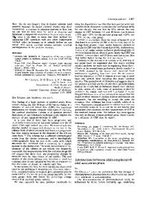
We start by taking Rb = 0.5Ra and focus on the case where A and B diffuse at the same speed 共D = 1兲. Figure 2共a兲 shows dispersion curves for Ra = 2.0, 5.0 共Rb = 1.0, 2.5兲 共case 1, Table I兲 for this case. Both the range of unstable wave numbers and the maximum growth rate max increase as Ra 共and hence Rb兲 is increased. This is to be expected as the density difference across the front, given by Eq. 共25兲, is then increasing. This is made clearer in Fig. 2共b兲 where we plot max against Ra. The rate of increase in max with Ra appears almost linear for the larger values of Ra. When Ra = 0, max = 0 as the system is then buoyantly marginally stable while the diffusive instability cannot set in as D = 1. 共In this and subsequent figures, • corresponds to values of parameters used for the numerical integrations.兲 For D ⬎ 1 共case 2, Table I and Fig. 3兲, both the range of unstable wave numbers and the maximum growth rates decrease for a given value of Ra, as can be seen in Fig. 3共a兲, comparing the dispersion curves for D = 1.0 and 2.0 at fixed Rayleigh numbers. In Fig. 3共b兲, the plot of max against D, again for Ra = 5.0, Rb = 2.5, shows that max decreases monotonically as D is increased from D = 1. There is also an associated decrease in the range of unstable wave numbers as D is increased. Thus the stabilizing effects of increased propagation speeds outweigh the destabilizing effect of differential diffusion 共at least for these parameter values兲. For D ⬍ 1 共case 3, Table I兲, we again have two competing effects, differential diffusion for D ⬍ 1 has a stabilizing influence on the RT instability 共see Fig. 1兲, however, the RD
0.12 0.1
5.0
0.08 0.06 0.04
2.0 0.02
k
0.0 -0.02 -0.04 0.0
0.1
0.2
0.3
0.4
0.5
0.6
(a) 0.12 max
0.1
0.08
0.06
0.04
0.02
Ra
0.0
(b) 0.0
0.5
1.0
1.5
2.0
2.5
3.0
3.5
4.0
4.5
5.0
FIG. 2. Stability results for the pure RT instability of ascending fronts obtained for D = 1.0. 共a兲 Dispersion curves for Ra = 2.0, 5.0, 共Rb = 1.0, 2.5兲. Expression 共41兲 for k small is shown by the broken line. 共b兲 A plot of max, the maximum value of the growth rate , against Ra 共with Rb = 0.5Ra兲.
fronts are also moving slower, which is favoring the destabilizing buoyancy effects. The competition between these effects leads to a nonmonotonous dependence of the dispersion curves on D 共see Fig. 4兲. When D is reduced from D = 1, the range of unstable wave numbers and the maximum growth rates increase, at least initially, probably because the RD front moves slower allowing the buoyancy effects to be more operative than when D = 1. However, there is a value of D at which both the range of unstable wave numbers and the maximum growth rates start to decrease as D is decreased further. This is due to the fact that the stabilizing influence of differential diffusion then takes over. This is illustrated in Fig. 4共a兲, showing dispersion curves for varying D at fixed Ra = 0.5 and more clearly in Fig. 4共b兲, where max is plotted against D. This figure suggests that max achieves its greatest value at D ⯝ 0.35 共for these values of Ra and Rb兲. In Fig. 4 and some other subsequent figures, we also plot as ⌬ growth rates obtained by following the early time linear growth of the transverse modulation of the interface as a function of
Downloaded 18 Mar 2009 to 164.15.128.33. Redistribution subject to AIP license or copyright; see http://jcp.aip.org/jcp/copyright.jsp
114502-6
J. Chem. Phys. 130, 114502 共2009兲
D’Hernoncourt, Merkin, and De Wit 0.008
0.12
0.3
0.1
1.0
0.006
0.5
0.08 0.06
0.004
2.0
0.15
0.04 0.002
0.02
1.0
k
0.0
k
0.0
-0.02 -0.002
-0.04
(a) 0.0
0.1
0.2
0.3
0.4
(a)
0.5
0.008
0.12
0.05
0.0
0.1
0.15
0.2
0.25
max
max
0.007
0.11 0.006
0.1 0.005
0.09
0.004
0.08
0.003
0.07
(b) 1.0
1.2
1.4
1.6
1.8
2.0
D
0.002
D
(b) 2.2
FIG. 3. Stabilizing influence of D ⬎ 1 on the RT instability of ascending fronts for Ra = 5.0, Rb = 2.5. 共a兲 Dispersion curves for D = 1.0, 2.0. 共b兲 A plot of max, the maximum value of the growth rate , against D.
time in the full nonlinear simulations of Eqs. 共10兲–共12兲. Good agreement between the results from the LSA and from the nonlinear simulations are obtained.43 At the smaller values of D, the system is also diffusionally unstable, diffusional instability requiring D ⬍ Dc ⯝ 0.424 for the cubic kinetics 关Eq. 共1兲兴. Figure 5共a兲 compares dispersion curves of the purely diffusional instability case 共D = 0.15, Ra = Rb = 0兲 to those obtained for parameters such that the system is both diffusionally and buoyantly unstable. For Ra = 0.5 the growth rates are comparable with those for the Ra = 0 case, though the range of unstable wave numbers is somewhat less. As Ra 共and hence Rb兲 is increased the maximum growth rate increases, though the range of unstable wave numbers does not appear to change significantly. In Fig. 5共b兲 max is plotted against Ra for D = 0.15, which shows that max has a minimum value at Ra ⯝ 0.2 before increasing with Ra. For larger values of Ra, max increases rapidly, soon becoming much larger than the diffusional instability value of max = 0.004 34 obtained for Ra = 0. Also plotted in Fig. 5共b兲 are the values of max for D = 1.0 for smaller values of Ra 关highlighting the small Ra part of Fig.
0.1
0.2
0.3
0.4
0.5
0.6
0.7
0.8
0.9
1.0
FIG. 4. Influence of D ⬍ 1 on the RT instability of ascending fronts for Ra = 0.5, Rb = 0.25. 共a兲 dispersion curves for D = 1.0, 0.5, 0.3, 0.15. 共b兲 A plot of max, the maximum value of the growth rate , against D. The values of max obtained directly from the growth of fingers at early times in full nonlinear simulations are shown by 䉭.
2共b兲兴 to compare with the values for D = 0.15. For small values of Ra the system is more unstable with D = 0.15, arising mainly from the fact that the system is also diffusionally unstable for this value of D 共max ⬎ 0 at Ra = 0兲, whereas with D = 1.0, it is stable at Ra = 0 共max = 0 at Ra = 0兲. However, the system with D = 1.0 becomes the more unstable one 共greater values of max兲 at Ra ⯝ 0.9. To understand the nonmonotonous character of the dependence of on Ra when D ⬍ Dc, we refer to the displaced particle argument of Fig. 6. The unstable diffusive character of the front when Ra = 0 is usually understood as follows:27 in the concave part of the perturbation as seen on Fig. 6 共upper part兲, A is diluted out of the perturbation. There is thus less reactant A ahead of the front, which slows down its progression favoring the growth in amplitude of the perturbation and destabilizing the front. On the contrary, the autocatalyst B gets concentrated ahead of the perturbation speeding up the front that tends to go back to its planar form, thus stabilizing the system. A diffusive instability is observed when the destabilizing diffusion of A wins over the stabilizing diffusion
Downloaded 18 Mar 2009 to 164.15.128.33. Redistribution subject to AIP license or copyright; see http://jcp.aip.org/jcp/copyright.jsp
114502-7
J. Chem. Phys. 130, 114502 共2009兲
Buoyancy and diffusion instabilities
0.007 0.006
A
Ra = 5
B
Rb = 2.5
A
Ra = 5
0.75
0.005 0.004
0.5
0.003 0.002 0.001
k
0.0 -0.001
(a)
0.0
0.05
0.1
0.15
0.2
0.25
0.3
0.35
0.4
max
FIG. 6. Displaced particle argument for D ⬍ 1 showing how the fact that Ra ⬎ Rb stabilizes the differential diffusive instability at least for small Rayleigh numbers as seen on Fig. 5.
The dispersion curves shown in Figs. 2共a兲, 3共a兲, and 4共a兲 have a similar form for small values of k. This leads us to obtain a solution of the LSA 关Eqs. 共20兲–共22兲兴 valid for small k.
0.008
0.006
0.15
2. Solution for small k
0.004
To obtain a solution of Eqs. 共20兲–共22兲 valid for small k, we expand
1.0 0.002
˜ + k2˜A + ¯ , A0 = ˜A0 + kA 1 2 Ra
0.0
(b) 0.0
0.1
0.2
0.3
0.4
0.5
0.6
0.7
0.8
0.9
˜ + k2˜B + ¯ , B0 = ˜B0 + kB 1 2
共26兲
1.0
FIG. 5. Stability results for the diffusionally unstable case for ascending fronts. 共a兲 Dispersion curves for D = 0.15, Ra = 0.5, 0.75 共with Rb = 0.5Ra兲. The pure diffusionally instability dispersion curve is shown by the broken curve 共D = 0.15, Ra = 0兲. 共b兲 max, the maximum value of the growth rate , plotted against Ra for D = 1.0 and 0.15. The values of max obtained from nonlinear simulations are shown by 䉭.
of B, i.e., when DA ⬎ DB and in practice when D ⬍ Dc. However, if Ra ⬎ Rb, A is denser than B, which then counteracts the diffusive growth of the perturbation. This stabilizing buoyancy effect decreases the growth rate of the diffusive instability for moderate values of Ra. However, when Ra is further increased, the standard RT instability takes over and the growth rate again becomes an increasing function of Ra 关see Fig. 5共b兲兴. The transition from density effects stabilizing the diffusive instability at moderate values of Ra and destabilizing buoyancy effects at larger Ra lead to the nonmonotonous character of the curve for D = 0.15 seen in Fig. 5共b兲. A comparison with a similar curve for D = 1 in Fig. 5共b兲, for which there are no diffusive instabilities, shows, as expected, that the larger values of max for small Ra and D ⬍ 1 are clearly related to the differential diffusivity of A and B. For Ra ⲏ 0.9, the system is more unstable for D = 1 than for D = 0.15 as D ⬍ 1 has a stabilizing effect on the RT instability as explained in Fig. 1. Below Ra ⯝ 0.2, the diffusive instability takes over so that the curve of max against Ra increases until the pure diffusive instability threshold is reached at Ra = 0.
u0 = kU1 + k2U2 + ¯ ,
= k 0 + k 2 1 + ¯ .
˜ , ˜B 兲 The equations for ˜A0 and ˜B0 have the solution 共A 0 0 = 共a⬘ , b⬘兲, where 共a , b兲 is the traveling wave solution given by Eqs. 共16兲 and 共17兲. At O共k兲 we have U1⬙ = 0 and we take U1 to be a, as yet ˜ , ˜B 兲 are then undetermined, constant. The equations for 共A 1 1 ˜A⬙ + cA ˜ ⬘ − b2˜A − 2abB ˜ = 共 + U 兲a⬘ , 1 1 0 1 1 1
共27兲
˜ ⬙ + cB ˜ ⬘ + b2˜A + 2abB ˜ = 共 + U 兲b⬘ . DB 1 1 0 1 1 1
共28兲
Now Eqs. 共27兲 and 共28兲 have a complementary function 共a⬘ , b⬘兲, which satisfies the 共homogeneous兲 boundary conditions given in Eq. 共23兲. Thus, any solution to Eqs. 共27兲 and 共28兲, which satisfies homogeneous boundary conditions, must also satisfy a compatibility condition. To determine this condition we follow35 and construct the adjoint problem 共U共兲 , V共兲兲 for Eqs. 共27兲 and 共28兲, namely, d c 共e U⬘兲 − b2共ecU − ec/DV兲 = 0, d 共29兲 d 共Dec/DV⬘兲 − 2ab共ecU − ec/DV兲 = 0, d subject to
Downloaded 18 Mar 2009 to 164.15.128.33. Redistribution subject to AIP license or copyright; see http://jcp.aip.org/jcp/copyright.jsp
114502-8
J. Chem. Phys. 130, 114502 共2009兲
D’Hernoncourt, Merkin, and De Wit
U,V → 0
as → ⫾ ⬁.
共30兲
A full derivation of this adjoint problem is given in Ref. 35. The compatibility condition is then, again from Ref. 35, 共0 + U1兲共I1 + I2兲 = 0, where I1 =
冕
⬁
eca⬘Ud,
共31兲
I2 =
−⬁
冕
⬁
ec/Db⬘Vd .
−⬁
It was seen in Ref. 35 that I1 + I2 ⫽ 0 except when D = 1, which is a degenerate case for the present analysis. Expression 共31兲 then gives
0 + U1 = 0,
˜ ,B ˜ and hence 共A 1 1兲 = K1共a⬘,b⬘兲
共32兲
for some constant K1. At O共k2兲 we then have U2⬙ = Raa⬘ + Rbb⬘ ,
共33兲
˜A⬙ + cA ˜ ⬘ − b2˜A − 2abB ˜ = 共 K + 1 + 兲a⬘ + a⬘U , 2 2 0 1 1 2 2 2 共34兲
buoyantly unstable, at least for sufficiently small wave numbers. The problem for D = 1 is somewhat simpler to deal with as the order of the system can be reduced since now a + b ⬅ 1, A0 + B0 ⬅ 0. An expansion analogous to that described above can be carried out, the end result still being Eq. 共41兲. Expression 共41兲 for k small is plotted in Fig. 2共a兲 共shown by a broken line兲 for the Ra = 5.0, Rb = 2.5 case, and shows good agreement, at least for small k, with the numerically determined values of . Result 共41兲 holds for upward propagating fronts. To consider downward propagating fronts, we need only change the sign of the terms on the right-hand side of Eq. 共10兲, corresponding to a change in sign of the buoyancy force term in Eq. 共3兲. Consequently for the LSA, there is a change in sign for the final terms in Eq. 共22兲. The result is that
⬃−
共Ra − Rb兲 k+ ¯ 2
for k small,
共42兲
showing that is negative for small wave numbers for downward propagating fronts, a situation which we now consider in more detail.
˜ ⬙ + cB ˜ ⬘ + b2˜A + 2abB ˜ = 共 K + D + 兲b⬘ + b⬘U . DB 2 2 0 1 1 2 2 2 共35兲 Equation 共33兲 gives U2⬘ = Raa + Rbb + L2
共36兲
for some constant L2. Clearly this does not satisfy the boundary conditions as → ⫾ ⬁ for any choice of L2. This means that outer regions are required in which these conditions are attained. We construct two outer regions, both with independent variable Y = k, one in Y ⬎ 0 and the other in Y ⬍ 0. In these regions A0 ⬅ 0 and B0 ⬅ 0 共at least to the order we are working兲 and in which we put u0 = kw, where w satisfies w⬙ − w = 0
in 0 ⬍ Y ⬍ ⬁
and in − ⬁ ⬍ Y ⬍ 0, 共37兲
subject to the matching conditions, from Eq. 共36兲, that w ⬃ U1 + 共Ra + L2兲Y + ¯ as Y → 0+ , w ⬃ U1 + 共Rb + L2兲Y + ¯
as Y → 0− .
共38兲
The solutions to Eq. 共37兲, which satisfies Eq. 共38兲, are w = U1e−Y
in Y ⬎ 0,
w = U 1e Y
in Y ⬍ 0.
共39兲
Applying the matching conditions 共38兲, at O共Y兲, in 共39兲 gives R a + L 2 = − U 1,
Rb + L2 = U1 .
共40兲
From Eqs. 共32兲 and 共40兲 it follows that 0 = 共Ra − Rb兲 / 2 and hence
⬃
共Ra − Rb兲 k+ ¯ 2
for k small,
共41兲
independent of D, as is seen in Figs. 3共a兲 and 4共a兲. Expression 共41兲 shows that upward propagating fronts are always
3. Downward propagating fronts
Relation 共41兲 between and k for k small indicates that upward propagating fronts will always be unstable for Ra ⬎ Rb 共cases 1–3, Table I兲, at least for sufficiently small wave numbers. For downward propagating fronts, the values of given by Eq. 共42兲 will be negative for small wave number k. This is readily understood for D = 1 for which the system is buoyantly stable featuring a stable density stratification of lighter products B over heavier reactant A 共case 4, Table I兲. For D ⬎ 1 and Ra ⬎ Rb 共case 5, Table I兲, the stabilizing effect of differential diffusion and the fact that the base state reaction front travels faster for D ⬎ 1 共which is unfavorable to the development of the RT instability兲 both make descending fronts even more stable than for D = 1. However, when D ⬍ 1, differential diffusion and the slower RD speed both act to destabilize the favorable density stratification 共case 6, Table I兲 and for D ⬍ Dc, the system is also diffusionally unstable. It may then be possible to destabilize the system and thus have ⬎ 0 over a finite range of nonzero wave numbers. This possibility can be seen in Fig. 7共a兲, where we give dispersion curves for Ra = 0.25, 0.5 共with D = 0.15 and ␣ = 0.5兲 for downward propagating fronts. For both values of Ra, there is a finite range of wave numbers over which ⬎ 0 and the system is unstable, even though ⬍ 0 for small k. Note that the maximum growth rates in this case are somewhat greater than those for the upward propagating reaction fronts 关compare the value of max for Ra = 0.5 in Fig. 7共a兲 with that in Fig. 5共a兲兴 and are also greater than for the pure diffusional instability case 共Ra = 0兲, shown in Fig. 5共a兲 by a broken line. The system becomes more unstable with increased values for max and a greater range of unstable wave numbers as Ra is increased 共at least for the values of Ra tried兲. This can be seen in Fig. 7共b兲, where we plot max against Ra for D = 0.15. This figure shows
Downloaded 18 Mar 2009 to 164.15.128.33. Redistribution subject to AIP license or copyright; see http://jcp.aip.org/jcp/copyright.jsp
114502-9
J. Chem. Phys. 130, 114502 共2009兲
Buoyancy and diffusion instabilities 0.025
0.014
0.5
0.012
0.02
max
0.01 0.008
0.015
0.25
0.006 0.01
0.004 0.002
k
0.0
D
0.0
-0.002
(a)
0.005
0.0
0.05
0.1
0.2
0.3
0.4
0.5
0.6
(a) 0.05
0.1
0.15
0.2
0.25
0.3
0.5 max
Ra 0.4
0.04
stable 0.03
0.3
0.02
0.2
0.01
0.1
unstable
Ra
0.0
(b) 0.0
0.2
0.4
0.6
0.8
1.0
1.2
1.4
0.0
1.6
FIG. 7. Stability results for the diffusionally unstable case for descending fronts. 共a兲 Dispersion curves for D = 0.15, Ra = 0.25, 0.5 共with Rb = 0.5Ra兲. The pure diffusionally instability dispersion curve is shown by the broken curve 共D = 0.15, Ra = 0兲. 共b兲 max, the maximum value of the growth rate , plotted against Ra. The values of max obtained directly from nonlinear simulations are shown by 䉭.
that max is somewhat greater in this case than for the upward propagating fronts 关compare with Fig. 5共b兲兴. The result that downward propagating fronts, which are buoyantly stable, can become more unstable than their buoyantly unstable ascending equivalent when they are diffusionally unstable is perhaps unexpected. The reason for this instability can be explained by the displaced particle argument described above and in Fig. 1 and results from the fact that having D ⬍ 1 gives a destabilizing influence on buoyancy effects for descending fronts when Ra ⬎ Rb.41 A related effect, seen when the buoyancy forces result from both concentration and temperature gradients, has already been shown to be able to destabilize a stratification of solute-light and hot products on top of solute-heavy and cold reactants in exothermic fronts.40 We examined this enhanced instability of downward propagating fronts in a little more detail. In Fig. 8共a兲 we plot max against D for Ra = 0.5 and descending fronts. The figure shows that max increases as D is decreased. max becomes
(b) 0.28
0.3
0.32
0.34
0.36
0.38
D
0.4
0.003 max
0.0025
0.002
0.0015
0.001
0.0005
Ra
0.0
(c)
0.0
0.2
0.4
0.6
0.8
1.0
1.2
FIG. 8. Influence of D ⬍ 1 on the RT instability of descending fronts for Ra = 0.5, Rb = 0.25. 共a兲 max plotted against D. The values of max obtained directly from nonlinear simulations are shown by 䉭. 共b兲 The values of Ra at which the system changes from being unstable to being stable plotted against D. 共c兲 max, plotted against Ra 共with Rb = 0.5Ra兲 for D = 0.28⬍ D1, illustrating that the system remains unstable for all Ra when D ⬍ D1.
zero at D ⯝ 0.285, with the system then being fully stable at larger D for this value of Ra, i.e., has ⬍ 0 for all k ⬎ 0. This latter point raises the question as to how the change in stability depends on the value of Ra. In Fig. 8共b兲 we plot the
Downloaded 18 Mar 2009 to 164.15.128.33. Redistribution subject to AIP license or copyright; see http://jcp.aip.org/jcp/copyright.jsp
114502-10
J. Chem. Phys. 130, 114502 共2009兲
D’Hernoncourt, Merkin, and De Wit TABLE II. Same as Table I in the case when Ra ⬍ Rb. Case
Direction
D
Buoy
Diff.
RD
Stability
Figure
7 8 9
Up Up Up
D=1 D⬎1 Dc ⬍ D ⬍ 1
+ + +
Neutral ⫺ +
Neutral + ⫺
9b 10 11 12
Up Down Down Down
D ⬍ Dc D=1 D⬎1 D⬍1
+ ⫺ ⫺ ⫺
⫺ Neutral + ⫺
⫺ Neutral + ⫺
Stable Stable Stable Lowered diffusional instability if D ⬍ Dc RT unstable Unstable ST chaos
10 9 11 12 and 13
values of Ra at which the system changes from being unstable to being fully stable against D, still with Rb = 0.5Ra. This figure shows that the region of instability 共as labeled on the figure兲 decreases as D is increased and strongly suggests that having D ⬍ Dc, i.e., having the system diffusionally unstable, is a necessary requirement for downward propagating fronts to become unstable through buoyancy effects when the products are lighter than the reactants 共Rb ⬍ Ra兲. Figure 8共b兲 also shows that there is a value D1 of D, with D1 ⯝ 0.284 such that, for D ⬍ D1, the system is always unstable for all values of Ra. Thus stability can be restored by making Ra sufficiently large 共i.e., increasing the stabilizing effect of having light B over heavy A兲 only for D in the range D1 ⬍ D ⬍ Dc. To illustrate this point further, max is plotted against Ra in Fig. 8共c兲 for D = 0.28, a value just below D1. This figure shows that max ⬎ 0 for all Ra, having a minimum value of max ⯝ 5 ⫻ 10−4 before increasing for larger values of Ra. For values of D ⬎ D1, we find that max decreases to zero for increasing Ra at the values shown in Fig. 8共b兲 and remains zero thereafter. C. Dispersion curves for Rb > Ra
We now consider those families of reactions where the products are heavier than the reactant, as in the CT system for example. For this situation we take ␣ = 2.0, i.e., Rb = 2Ra.
We now examine what happens to ascending fronts when D ⫽ 1. A displaced particle argument similar to the one given in Fig. 1 suggests that upward propagating fronts will be even more stable 共i.e., have growth rates even more negative兲 for D ⬍ 1 as differential diffusion is now a stabilizing mechanism 共case 9, Table II兲. However, when D ⬍ Dc, the diffusional instability becomes operative, at least for small values of Ra and Rb 共small density changes across the front兲. Hence we might expect that the dispersion curves for upward propagating fronts will have, at least for small Ra 共where the buoyantly stabilizing influence of light A over heavy B is not too important兲, a range of unstable wave numbers where ⬎ 0, though they will start with ⬍ 0 from expression 共41兲. We illustrate this possibility in Fig. 10 where we give dispersion curves for upward propagating fronts with D = 0.15. For Ra = 0.05 共Rb = 0.1兲 the LSA suggests that the front is stable. However, for Ra = 0.025 共Rb = 0.05兲 there is a range of wave numbers for which ⬎ 0, indicating that the front is unstable. The transition from stability to instability is at Ra ⯝ 0.0365. If we compare, for example, the maximum growth rate max for Ra = 0.025 with that for the purely diffusional instability 关Fig. 5共b兲兴, we see that it is somewhat smaller, by a factor of approximately 0.3. This emphasizes the fact that the stabilizing effect of the buoyancy forces has here a much stronger influence than the destabilization due to differential
1. Upward propagating fronts 0.3
In this case, when D = 1, it is the downward propagating fronts that are buoyantly unstable 共case 10, Table II兲, with the upward propagating fronts being buoyantly stable 共case 7, Table II兲, as can also be expected from Eqs. 共41兲 and 共42兲. In all the cases tried for D = 1, the LSA does indeed show that upward propagating fronts are stable and that downward propagating fronts are unstable. We illustrate this by the dispersion curves for D = 1.0 and Ra = 1.0, 2.5, 5.0 shown in Fig. 9. A point to note from this figure is that, for a given value of Ra, the growth rates are somewhat higher than in the previous case where Rb = 0.5Ra 关Fig. 2共a兲兴. This might be expected as, from Eq. 共25兲, the same value of Ra corresponds to a greater change in density across the front in the present case, where ␣ = 2 than in the one depicted in Fig. 2共a兲, where ␣ = 0.5. If we consider values of Ra and ␣, which give the same density change across the front, for example, Ra = 1.0, ␣ = 2 in Fig. 9 with Ra = 2.0, but ␣ = 0.5 in Fig. 2共a兲, then we see comparable growth rates, as might be expected.
5.0
0.25 0.2 0.15 0.1
2.5 0.05
1.0 k
0.0 -0.05 -0.1 0.0
0.1
0.2
0.3
0.4
0.5
0.6
0.7
0.8
FIG. 9. Dispersion curves for D = 1.0 and descending fronts for the case Rb ⬎ Ra 共Rb = 2Ra with Ra = 1.0, 2.5, 5.0兲.
Downloaded 18 Mar 2009 to 164.15.128.33. Redistribution subject to AIP license or copyright; see http://jcp.aip.org/jcp/copyright.jsp
114502-11
J. Chem. Phys. 130, 114502 共2009兲
Buoyancy and diffusion instabilities 0.04
0.001
0.025
0.2
0.0005
0.03
k
0.0
0.02 -0.0005
0.05
0.01
-0.001
0.1
k
-0.0015
0.0
0.05 -0.002
0.0365 -0.01
-0.0025 -0.003
-0.02 0.0
0.05
0.1
0.15
0.2
0.25
0.3
0.0
0.1
0.2
0.3
0.4
0.5
0.6
0.7
0.8
(a) FIG. 10. Dispersion curves for D = 0.15 共diffusionally unstable case兲 and Ra = 0.025, 0.0365, 0.05 共with Rb = 2Ra兲 for ascending fronts.
diffusion. This is in sharp contrast with the previous Ra ⬎ Rb case for buoyantly stable descending fronts 共case 6, Table I兲 illustrated in Figs. 7 and 8. 2. Downward propagating fronts
We now consider descending fronts for Rb ⬎ Ra and D ⫽ 1. In this case, the front is RT unstable as heavy products are lying on top of lighter reactants. If D ⬎ 1 共case 11, Table II兲, differential diffusion has a stabilizing influence on the RT instability. Both max and the range of unstable wave numbers decrease as D is increased from D = 1.0, as is illustrated in Fig. 11. The most unstable case is the one for which all three effects 共buoyancy, differential diffusion and influence of D ⫽ 1 on the RD speed兲 are destabilizing 共case 12, Table II兲 and this most unstable configuration occurs for descending fronts when Rb ⬎ Ra and D ⬍ 1. This is confirmed in Fig. 12共a兲 featuring dispersion curves for descending, buoyantly 0.01
max
0.009
0.008
0.007
0.006
0.005
0.004
D 0.003 1.0
1.2
1.4
1.6
1.8
2.0
2.2
FIG. 11. max, the maximum value of the growth rate , plotted against D for D ⱖ 1 and for downward propagating fronts and the case Rb ⬎ Ra with Ra = 0.5, Rb = 1.0.
0.06
max
0.05
0.04
0.03
0.02
0.01
Ra
0.0
(b) 0.0
0.05
0.1
0.15
0.2
0.25
0.3
FIG. 12. Stability results for descending fronts when the system is both diffusionally and buoyantly unstable. 共a兲 dispersion curves for D = 0.15 and Ra = 0.05, 0.1, 0.2 共with Rb = 2Ra兲. 共b兲 max, the maximum value of the growth rate , plotted against Ra. The values of max obtained directly from the nonlinear simulations are shown by 䉱.
and diffusively unstable fronts for D = 0.15 and Ra = 0.05, 0.1, 0.2. Values of max as a function of Ra are plotted in Fig. 12共b兲, showing a rapid 共apparently linear兲 increase in max as Ra is increased. In this particular case, we found it more difficult to compute the dispersion curves than previously 共in all other cases the calculations proceeded very easily兲. Even when taking very small increments in the wave number, we were unable to get the numerical scheme to converge, especially for small values of k. This might be explained by the much larger values of found in this case than for the Ra ⬎ Rb case. For Ra = 0.2 共Rb = 0.4兲, Fig. 12共a兲, we find max ⯝ 0.0383 compared to a value of max ⯝ 0.0033 关Fig. 5共b兲兴. Even allowing for the different changes in density, max ⯝ 0.0040 for Ra = 0.4 in Fig. 5共b兲. In general, the values of max appear to be at least an order of magnitude greater for this case. Further to this point, the range of unstable wave numbers is considerably greater for this case 共compare Fig. 12共a兲 with Fig. 5共a兲 or Fig. 7共a兲兲. The strong destabilizing effect of the differential diffu-
Downloaded 18 Mar 2009 to 164.15.128.33. Redistribution subject to AIP license or copyright; see http://jcp.aip.org/jcp/copyright.jsp
114502-12 0.045
J. Chem. Phys. 130, 114502 共2009兲
D’Hernoncourt, Merkin, and De Wit
max
0.04 0.035 0.03 0.025 0.02 0.015 0.01 0.005
D
0.0 0.2
0.3
0.4
0.5
0.6
0.7
0.8
0.9
1.0
FIG. 13. max, the maximum value of the growth rate , plotted against D for D ⱕ 1, downward propagating fronts in the case Rb ⬎ Ra with Ra = 0.25, Rb = 0.5. The values of max obtained directly from the nonlinear simulations are shown by 䉭.
sion instability on downward propagating fronts when Ra ⬍ Rb can clearly be seen in Fig. 13, where we plot max against D for Ra = 0.25, Rb = 0.5 共␣ = 2.0兲. This figure shows a sharp increase in max around the point where D = Dc. The range of unstable wave numbers is also greatly increased from 0 ⬍ k ⬍ 0.096 for D = 1.0 to 0 ⬍ k ⬍ 0.731 for D = 0.2. IV. CONCLUSIONS
In autocatalytic reaction fronts where there is more than one key chemical species, it is common for the reactant A and autocatalytic product B of the reaction to have different diffusion coefficients 共i.e., D = DB / DA ⫽ 1兲 and also to have different densities. Here we examined by a LSA the mutual influence of such differential diffusion and RT fingering instabilities of chemical fronts due to an unfavorable density stratification in a gravity field. We have shown that the problem can be classified into 12 different cases 共Tables I and II兲 depending whether the front is ascending or descending in the gravity field, whether the Rayleigh number Ra of the reactant is smaller or larger than the Rayleigh number Rb of the products, and whether D = 1, D ⬍ 1, or D ⬎ 1. If the reactant diffuses sufficiently faster than the product 共D ⬍ Dc兲, the system can also be unstable through a diffusive instability giving rise to a cellular deformation of the front. The stability properties can be understood as the result of three effects: 共i兲 fronts are buoyantly unstable when heavier solution lies on top of a lighter one in the gravity field, 共ii兲 D ⬎ 1 共D ⬍ 1兲 is having a destabilizing 共stabilizing兲 effect on buoyantly unstable ascending fronts while destabilizing 共stabilizing兲 the descending fronts when Ra ⬎ Rb 共the reverse is true when Ra ⬍ Rb兲, and 共iii兲 fronts travel faster for increasing values of D, which is unfavorable to the RT instability. As a corollary, slower fronts obtained when D is decreased below one are more prone to favor the RT instability. As a consequence of the competition or cooperation between these three effects, various stability scenarios have been highlighted from the LSA 共giving dispersion curves i.e., the
growth rate of the perturbation as a function of their wave number k, for various values of the parameters兲, as well as from analytical results for small k. This allowed to understand what kind of stability properties are to be expected if a pair of counter-propagating fronts are generated in the middle of a Hele–Shaw cell when differential diffusion phenomena are present in addition to possible buoyancy-driven instabilities. When the reactants are heavier than the products, as in the IAA reaction for example, then, for D = 1, only the ascending front is buoyantly unstable and no diffusive instability can take place. If D ⬎ 1, the RT instability of the ascending fronts will be less efficient as D ⬎ 1 has a stabilizing influence, the descending front remaining stable. The most striking effect of differential diffusion comes however when D ⬍ 1. In this case, for ascending fronts, the most unstable growth rate max varies nonmonotonically with D when D is decreased below one while descending fronts have their diffusive instability magnified when D ⬍ Dc. Buoyancy effects in this case enhance the cellular deformation due to a diffusive instability. When the products are heavier than the reactants, as in the CT reaction, the stability scenarios are quite different. For D = 1, the ascending front is now buoyantly stable while the descending one features a hydrodynamic RT fingering instability. If D ⬎ 1, differential diffusion cannot destabilize an ascending front but can reduce the strength of the RT instability of descending fronts. When D ⬍ Dc, the diffusive instability of ascending fronts is lowered by buoyancy effects. The most interesting situation occurs on descending fronts when D ⬍ Dc ⬍ 1, in which case all effects combine to strongly destabilize the front. The classification given in this article should allow us to predict all possible stability conditions of autocatalytic fronts where the density either decreases or increases across the front and the two key species diffuse at different rates. In order to give insight into the spatiotemporal dynamics that might be observed experimentally in the various stability scenarios studied here, numerical simulations of the full nonlinear problem have been performed and are detailed in a companion paper.43 ACKNOWLEDGMENTS
A.D. thanks A. Tóth and D. Horváth for fruitful discussions and acknowledges financial support from FNRS, Prodex and the Communauté franaise de Belgique 共ARC program兲. J.D. benefitted from a FRIA Ph.D. fellowship. 1
J. A. Pojman, I. R. Epstein, T. J. McManus, and K. Showalter, J. Phys. Chem. 95, 1299 共1991兲. 2 J. Masere, D. A. Vasquez, B. F. Edwards, J. W. Wilder, and K. Showalter, J. Phys. Chem. 98, 6505 共1994兲. 3 M. R. Carey, S. W. Morris, and P. Kolodner, Phys. Rev. E 53, 6012 共1996兲. 4 M. Böckmann and S. C. Müller, Phys. Rev. Lett. 85, 2506 共2000兲. 5 J. Martin, N. Rakotomalala, D. Salin, and M. Böckmann, Phys. Rev. E 65, 051605 共2002兲. 6 M. Böckmann and S. C. Müller, Phys. Rev. E 70, 046302 共2004兲. 7 M. C. Rogers and S. W. Morris, Phys. Rev. Lett. 95, 024505 共2005兲. 8 L. Sebestikova, J. D’Hernoncourt, M. J. B. Hauser, S. C. Müller, and A. De Wit, Phys. Rev. E 75, 026309 共2007兲.
Downloaded 18 Mar 2009 to 164.15.128.33. Redistribution subject to AIP license or copyright; see http://jcp.aip.org/jcp/copyright.jsp
114502-13 9
J. Chem. Phys. 130, 114502 共2009兲
Buoyancy and diffusion instabilities
I. P. Nagy, A. Keresztessy, J. A. Pojman, G. Bazsa, and Z. Noszticzius, J. Phys. Chem. 98, 6030 共1994兲. 10 A. Keresztessy, I. P. Nagy, G. Bazsa, and J. A. Pojman, J. Phys. Chem. 99, 5379 共1995兲. 11 J. A. Pojman, A. Komlósi, and I. P. Nagy, J. Phys. Chem. 100, 16209 共1996兲. 12 M. Matalon and B. J. Matkowsky, Combust. Sci. Technol. 34, 295 共1983兲. 13 N. Vladimirova and R. Rosner, Phys. Rev. E 67, 066305 共2003兲. 14 J. D’Hernoncourt, A. Zebib, and A. De Wit, Chaos 17, 013109 共2007兲. 15 D. Horváth, T. Bánsági, Jr., and A. Tóth, J. Chem. Phys. 117, 4399 共2002兲. 16 T. Bánsági, Jr., D. Horváth, Á. Tóth, J. Yang, S. Kalliadasis, and A. De Wit, Phys. Rev. E 68, 055301 共2003兲. 17 T. Bánsági, Jr., D. Horváth, and Á. Tóth, Phys. Rev. E 68, 026303 共2003兲. 18 T. Bánsági, Jr., D. Horváth, and Á. Tóth, Chem. Phys. Lett. 384, 153 共2004兲. 19 T. Bánsági, Jr., D. Horváth, and Á. Tóth, J. Chem. Phys. 121, 11912 共2004兲. 20 T. Rica, D. Horváth, and Á. Tóth, Chem. Phys. Lett. 408, 422 共2005兲. 21 D. Horváth, S. Tóth, and Á. Tóth, Phys. Rev. Lett. 97, 194501 共2006兲. 22 T. Tóth, D. Horváth, and Á. Tóth, Chem. Phys. Lett. 442, 289 共2007兲. 23 T. Tóth, D. Horváth, and Á. Tóth, J. Chem. Phys. 127, 234506 共2007兲. 24 G. Bazsa and I. R. Epstein, J. Phys. Chem. 89, 3050 共1985兲. 25 I. Nagypál, G. Bazsa, and I. R. Epstein, J. Am. Chem. Soc. 108, 3635 共1986兲. 26 J. A. Pojman, I. P. Nagy, and I. R. Epstein, J. Phys. Chem. 95, 1306 共1991兲. 27 D. Horváth, V. Petrov, S. K. Scott, and K. Showalter, J. Chem. Phys. 98, 6332 共1993兲. 28 A. Malevanets, A. Careta, and R. Kapral, Phys. Rev. E 52, 4724 共1995兲. 29 D. Horváth and K. Showalter, J. Chem. Phys. 102, 2471 共1995兲. 30 D. Horváth and A. Tóth, J. Chem. Phys. 102, 2471 共1995兲. 31 A. Tóth, I. Lagzi, and D. Horváth, J. Phys. Chem. 100, 14837 共1996兲.
A. Tóth, B. Veisz, and D. Horváth, J. Phys. Chem. A 102, 5157 共1998兲. D. Horváth and A. Tóth, J. Chem. Phys. 108, 1447 共1998兲. 34 M. Fuentes, M. N. Kuperman, and P. De Kepper, J. Phys. Chem. A 105, 6769 共2001兲. 35 J. H. Merkin and I. Z. Kiss, Phys. Rev. E 72, 026219 共2005兲. 36 J. H. Merkin and H. Ševčíková, Phys. Chem. Chem. Phys. 1, 91 共1999兲. 37 J. Yang, A. D’Onofrio, S. Kalliadasis, and A. De Wit, J. Chem. Phys. 117, 9395 共2002兲. 38 D. Lima, A. D’Onofrio, and A. De Wit, J. Chem. Phys. 124, 014509 共2006兲. 39 J. D’Hernoncourt, A. De Wit, and A. Zebib, J. Fluid Mech. 576, 445 共2007兲. 40 J. D’Hernoncourt, A. Zebib, and A. De Wit, Phys. Rev. Lett. 96, 154501 共2006兲. 41 J. D’Hernoncourt, J. H. Merkin, and A. De Wit, Phys. Rev. E 76, 035301 共2007兲. 42 J. Yuan, Y. Ju, and C. K. Law, Combust. Flame 144, 386 共2006兲. 43 J. D’Hernoncourt, J. Merkin, and A. De Wit, J. Chem. Phys. 130, 114503 共2009兲. 44 A. B. Tayler, Mathematical Models in Applied Mechanics 共Oxford Applied Mathematics and Computing Science Series, Clarendon Press, Oxford, 1986兲. 45 J. Billingham and D. J. Needham, Philos. Trans. R. Soc. London, Ser. A 334, 1 共1991兲. 46 J. Billingham and D. J. Needham, Dyn. Stab. Syst. 6, 33 共1991兲. 47 J. D’Hernoncourt, J. Merkin, and A. De Wit, J. Chem. Phys. 126, 104504 共2007兲. 48 A. De Wit, Phys. Rev. Lett. 87, 054502 共2001兲. 49 D. A. Vasquez, J. W. Wilder, and B. F. Edwards, J. Chem. Phys. 104, 9926 共1996兲. 50 M. Garbey, A. Taik, and V. Volpert, Q. Appl. Math. 56, 1 共1998兲. 51 B. McCaughey, J. A. Pojman, and C. Simmons, Chaos 8, 520 共1998兲. 52 Y. Wu, D. A. Vasquez, B. F. Edwards, and J. W. Wilder, Phys. Rev. E 51, 1119 共1995兲. 53 Numerical Algorithms Group, Web address: http://www.nag.co.uk/. 32 33
Downloaded 18 Mar 2009 to 164.15.128.33. Redistribution subject to AIP license or copyright; see http://jcp.aip.org/jcp/copyright.jsp