Interaction Force Fields for Molecular Mechanics and Molecular Dynamics Simulations Tahir Cagin
Molecular Modeling • • • • •
Electrons Atoms Segments Domains Continuum
Multiscale hierarchy of modeling time
ELECTRONS
ATOMS
DOMAINS
GRIDS
hours
Continuum (FEM)
seconds microsec nanosec
MESO First principles Force Fields
MD
picosec
femtosec
QM
Å
nm
micron
mm
meters
distance
A molecular Model of DNA
Molecular Model of a Solid
Force Fields • van der Waals interactions • Metal force fields – many body effects/electronic effects • Ligancy, ionicity/covalency • Covalent interactions • Chemical Reactions Finally – compliance/consistency/transferability
Force Fields • Simple Noble Gas Solid/Liquid/Gases • Metals and Alloys • Oxides, Carbides, Nitrides – Ceramics, Zeolites, Clays, Minerals • Organic Molecules, liquids, solids • Polymers, Composites • Proteins, Nucleic Acids And more importantly: Interfaces of any of the above
Valence Force Fields AMBER, Assisted Model Building and Energy Refinement AMBER/OPLS CHARMM, Chemistry at HARvard Macromolecular Mechanics DISCOVER, force fields of the Insight/Discover DREIDING, force fields of POLYGRAF/BIOGRAF GROMOS, GROningen MOlecular Simulation package MM2/MM3/MM4 , Allinger molecular mechanics FF MMFF94, the Merck Molecular Force Field Tripos, the force field of the Sybyl molecular modeling program UFF, Universal Force Fields of POLYGRAF/BIOGRAF/Cerius
DREIDING/UFF/References •Mayo S L, Olafson B D, Goddard W A, “DREIDING - A Generic Force-field For Molecular Simulations,” J Phys Chem 94 8897-8909 1990 •Rappe A K, Casewit C J, Colwell K S, et al. UFF, A Full Periodic-table Force-field For Molecular Mechanics And Molecular-dynamics Simulations J Am Chem Soc 114 10024-10035 1992 •Casewit C J, Colwell K S, Rappe A K, Application Of A Universal Force-field To Main Group Compounds J Am Chem Soc 114: 10046-10053 1992
Force Fields hb
Interaction types • Non Bonded Interactions • Electrostatics • van der Waals interactions • Valence Interactions • Bond Stretch • Angle Bending • Torsion/Dihedrals/Improper Torsions • 4+ body interactions • Special Interactions • Hydrogen bonding • Constraints
Non Bonded Interactions ELECTROSTATICS Electrostatics describes the force resulting from the interaction between two charged particles. The electrostatic energy between two atoms i and j is described by Coulomb's Law as
qi = charge of atom i; qj = charge of atom j = Dielectric constant , the vector from atom i to atom j = length of
, distance between atoms i and j
Non Bonded Interactions The van der Waals energy between two atoms i and j is described by
where A = Repulsion constant B = Attraction constant = distance between atoms i and j
Valence Interactions The energy of a bond between atoms i and j is given by
k = spring constant = distance between atoms i and j r0 = equilibrium distance of the bond The energy of such angle bending between atoms i, j, and k is given by
= force constant this angle-bending type = calculated angle between the vector i and j and vector k and j. 0 = equilibrium value of the bond angle
Dihedrals/Improper Torsions Dihedral and improper bonds model the interaction between 4 bonded atoms. They are modeled by an angular spring between the planes formed by the first 3 atoms and the second 3 atoms. The energy for a dihedral or improper between atoms i, j, k, and l is given by
k = force constant = angle between the plane formed by atoms (i, j, k) and the plane formed by atoms (j, k, l) n = periodicity of the bond specified in the parameter file for this bond type = phase shift
Harmonic Constraints Harmonic constraints provide a mechanism for holding certain parts of a molecule relatively immobile during a simulation. For instance: it allows specific atoms to be held at a reference position. The energy for an atom i that is constrained is
ki = force constant defined for atom i = current position of atom I = reference position atom i is constrained to
Evaluating Non Bond Interactions • Exclusion issues •Finite Systems • All non bond interactions are evaluated • Cut off distances are used • Direct Cut off • Shifted Energy • Shifted Force • Splines (continuity issues) • Screening issues • Infinite Systems • Cut offs • Minimum Image • Ewald/PME/FMM methods
Splines/Switching Functions For van der Waals interactions, the energy is modified as
switching function defined by
inner cutoff value for switching outer cutoff value for switching
Exclusions of Valence Interactions 4 2
1
3 5
The bonded terms are excluded in evaluating non bond interactions Bond stretch terms: 1-2; 2-3; 3-4; 4-5 Angle bend terms : 1-3; 2-4; 3-5 Optional exclusion for torsion terms: 1-4; 2-5 scale : 0 exclude scale : 0.5 as in AMBER scale : 1 include
AMBER/References •Cornell, W. D., Cieplak, P., Bayly, C. I., Gould, I. R., Merz, K. M. Jr., Ferguson, D. M. Spellmeyer, D. C., Fox, T., Caldwell, J. W., and Kollman, P. A. (1995) A second generation force field for the simulation of proteins, nucleic acids and organic molecules, J. Am. Chem. Soc. 117, 5179-5197. •Pearlman, D. A., Case, D. A., Caldwell, J. C., Seibel, G. L., Singh, U. C., Weiner, P., & Kollman, P. A., (1991) AMBER 4.0, University of California, San Francisco. •Weiner, P. K., & Kollman, P. A., (1981) AMBER: Assisted Model Building with Energy Refinement. A General Program for Modeling Molecules and Their Interactions, J. Comp. Chem. 2, 287-303. •Weiner, S.J., Kollman, P.A., Case, D.A., Singh, U.C., Ghio, C., Alagona, G., Profeta, S., Jr., Weiner, P.K. (1984) A new force field for molecular mechanical simulation of nucleic acids and proteins. J. Am. Chem. Soc. 106, 765-784. •Weiner, S. J., Kollman, P. A., Nguyen, D. T., and Case, D. A., (1986) "An All Atom Force Field for Simulations of Proteins and Nucleic Acids," J. Comp. Chem. 7, 230252.
OPLS/References •Damm, W., A. Frontera, J. Tirado-Rives and W. L. Jorgensen (1997) "OPLS All-Atom Force Field for Carbohydrates," J. Comp. Chem. 18, 1955-1970. Jorgensen, W. L.; Maxwell, D. S. and Tirado-Rives, J. (1996) "Development and Testing of the OPLS AllAtom Force Field on Conformational Energetics and Properties of Organic Liquids" J. Am. Chem. Soc., 118, 11225-11236. •Jorgensen, W. L., & Tirado-Rives, J.,(1988) The OPLS Potential Functions for Proteins. Energy Minimization for Crystals of Cyclic Peptides and Crambin, J. Am. Chem. Soc. 110, 1657-1666. •Kaminski, G., Duffy, E. M. Matsui, T., and Jorgensen, W. L. (1994) J. Phys. Chem. 98, 13077-13082.
CHARMM/References •Brooks, B.R., Bruccoleri, R.E., Olafson, B.D., States, D.J., Swaminathan, S., Karplus, M. (1983) CHARMM: A program for macromolecular energy, minmimization, and dynamics calculations. J. Comp. Chem. 4, 187-217. Feller et al.,(1997) Molecular Dynamics Simulation of Unsaturated Lipids at Low Hydration: Parameterization and Comparison with Diffraction Studies. Biophys. J. 73, 2269-2279 •MacKerell, A D ; Bashford, D; Bellott, M; Dunbrack, R L; Eva seck, J D; Field, M J; Fischer, S; Gao, J; Guo, H; Ha, S; JosephMcCarthy, D; Kuc nir, L; Kuczera, K; Lau, F T K; Mattos, C; Michnick, S; Ngo, T; Nguyen, D T; Pro hom, B; Reiher, W E; Roux, B; Schlenkrich, M; Smith, J C; Stote, R; Straub, J; W tanabe, M; WiorkiewiczKuczera, J; Yin, D; Karplus, M (1998) All-atom empirical potential for molecular modeling and dynamics studies of proteins. J. Phys. Chem., B 102, 3586-3617 •Mackerell A D ; Wiorkiewiczkuczera J; Karplus, M (1995) An all-atom empirical energy function for the simulation of nucleic acids. J. Amer. Chem. Soc.117, 11946-11975 •Momany, F. A., & Rone, R., (1992) Validation of the General Purpose QUANTA 3.2/CHARMm Force Field, J. Comp. Chem. 13, 888-900. •Pavelites, J. J., J. Gao, P.A. Bash and A. D. Mackerell, Jr. (1997) "A Molecular Mechanics Force Field for NAD+, NADH, and the Pyrophosphate Groups of Nucleotides," J. Comp. Chem. 18, 221-239. •Schlenkrich et al. (1996), Empirical Potential Energy Function for Phospholipids: Criteria for Parameter Optimization and Applications in "Biological Membranes: A Molecular Perspective from Computation and Experiment," K.M. Merz and B. Roux, Eds. Birkhauser, Boston, pp 31-81, 1996
DISCOVER/References •Dauber-Osguthorpe, P.; Roberts, V. A.; Osguthorpe, D. J.; Wolff, J.; Genest, M.; Hagler, A. T. (1988) "Structure and energetics of ligand binding to proteins: E. coli dihydrofolate reductase- trimethoprim, a drug-receptor system", Proteins: Structure, Function and Genetics, 4, 31-47. •Hagler, A. T.; Ewig, C. S. "On the use of quantum energy surfaces in the derivation of molecular force fields", Comp. Phys. Comm., 84, 131-155 (1994). •Hwang, M.-J.; Stockfisch, T. P.; Hagler, A. T. "Derivation of Class II force fields. 2. Derivation and characterization of a Class II force field, CFF93, for the alkyl functional group and alkane molecules", J. Amer. Chem. Soc., 116, 2515-2525 (1994). •Maple, J. R.; Hwang, M.-J.; Stockfisch, T. P.; Dinur, U.; Waldman, M.; Ewig, C. S; Hagler, A. T. "Derivation of Class II force fields. 1. Methodology and quantum force field for the alkyl functional group and alkane molecules", J. Comput. Chem., 15, 162-182 (1994a). •Maple, J. R.; Hwang, M.-J.; Stockfisch, T. P.; Hagler, A. T. "Derivation of Class II force fields. 3. Characterization of a quantum force field for the alkanes", Israel J. Chem., 34, 195 -231 (1994b).
Gromos/References •Hermans, J., Berendsen, H. J. C., van Gunsteren, W. F., & Postma, J. P. M., (1984) "A Consistent Empirical Potential for Water-Protein Interactions," Biopolymers 23, 1 Ott, K-H., B. Meyer (1996) "Parametrization of GROMOS force field for oligosaccharides and assessment of efficiency of molecular dynamics simulations," J Comp Chem 17, 1068-1084> •van Gunsteren, W. F., X. Daura and A.E. Mark (1997) "The GROMOS force field" in Encyclopaedia of Computational Chemistry ()
MM2/MM3/MM4/References •Lii, J-H., & Allinger, N. L. (1991) The MM3 Force Field for Amides, Polypeptides and Proteins, J. Comp. Chem. 12, 186-199. •Lii, J-H., & Allinger, N. L. (1998) Directional Hydrogen Bonding in the MM3 Force Field. II. J. Comp. Chem. 19, 1001-1016. •Allinger, N. L., K. Chen, and J-H Lii (1996) "An Improved Force Field (MM4) for Saturated Hydrocarbons," J. Comp. Chem. 17, 642-668. Allinger, N. L., K. Chen, J. A. Katzenellenbogen, S. R. Wilson and G. M. Anstead (1996) "Hyperconjugative Effects on Carbon-Carbon Bond Lengths in Molecular Mechanics (MM4)" J. Comp. Chem. 17, 747-755. •Allinger, N. L., and Y. Fan (1997) "Molecular Mechanics Studies (MM4) of Sulfides and Mercaptans," J. Comp. Chem.18, 1827-1847. •Nevens, N., K. Chen and N. L. Allinger (1996) "Molecular Mechanics (MM4) Calculations on Alkenes," J. Comp. Chem. 17, 669-694. •Nevins, N., J-H. Lii and N.L. Allinger (1996) "Molecular Mechanics (MM4) Calculations on Conjugated Hydrocarbons," J. Comp. Chem. 17, 695-729. •Nevins, N., and N. L. Allinger (1996) "Molecular Mechanics (MM4) Vibrational Frequency Calculations for Alkenes an Conjugated Hydrocarbons," J. Comp. Chem. 17, 730-746.
MM2/MM3/MM4/References •Lii, J-H., & Allinger, N. L. (1991) The MM3 Force Field for Amides, Polypeptides and Proteins, J. Comp. Chem. 12, 186-199. •Lii, J-H., & Allinger, N. L. (1998) Directional Hydrogen Bonding in the MM3 Force Field. II. J. Comp. Chem. 19, 1001-1016. •Allinger, N. L., K. Chen, and J-H Lii (1996) "An Improved Force Field (MM4) for Saturated Hydrocarbons," J. Comp. Chem. 17, 642-668. Allinger, N. L., K. Chen, J. A. Katzenellenbogen, S. R. Wilson and G. M. Anstead (1996) "Hyperconjugative Effects on Carbon-Carbon Bond Lengths in Molecular Mechanics (MM4)" J. Comp. Chem. 17, 747-755. •Allinger, N. L., and Y. Fan (1997) "Molecular Mechanics Studies (MM4) of Sulfides and Mercaptans," J. Comp. Chem.18, 1827-1847. •Nevens, N., K. Chen and N. L. Allinger (1996) "Molecular Mechanics (MM4) Calculations on Alkenes," J. Comp. Chem. 17, 669-694. •Nevins, N., J-H. Lii and N.L. Allinger (1996) "Molecular Mechanics (MM4) Calculations on Conjugated Hydrocarbons," J. Comp. Chem. 17, 695-729. •Nevins, N., and N. L. Allinger (1996) "Molecular Mechanics (MM4) Vibrational Frequency Calculations for Alkenes an Conjugated Hydrocarbons," J. Comp. Chem. 17, 730-746.
MMFF94/References •Halgren, T. A. (1992) J. Am. Chem. Soc. 114, 7827-7843. Halgren, T. A. (1996) "Merck Molecular Force Field. I. Basis, Form, Scope, Parameterization and Performance of MMFF94," J. Comp. Chem 17, 490-519. •Halgren, T. A. (1996) "Merck Molecular Force Field. II. MMFF94 van der Waals and Electrostatic Parameters for Intermolecular Interactions," J. Comp. Chem. 17, 520-552. •Halgren, T. A. (1996) "Merck Molecular Force Field. III. Molecular Geometrics and Vibrational Frequencies for MMFF94," J. Comp. Chem. 17, 553-586. •Halgren, T. A., and Nachbar, R. B. (1996) "Merck Molecular Force Field. IV. Conformational Energies and Geometries," J. Comp. Chem. 17, 587-615. •Halgren, T. A. (1996) "Merck Molecular Force Field. V. Extension of MMFF94 using Experimental Data, Additional Computational Data and Empirical Rules," J. Comp. Chem. 17, 616-641.
Molecular Dynamics
Tahir Cagin
Summary • Molecular Dynamics Methods – Equilibrium Molecular Dynamics Methods • Standard MD • Extended Hamiltonian Methods • Coarse Grain Methods
– Non Equilibrium Molecular Dynamics Methods • Steady State MD • Synthetic Hamiltonian NEMD Methods
• • • •
Molecular Dynamics Introduction Statistical Mechanics and Ensembles Static Property Calculations Dynamic Property Calculations from Equilibrium and NE MD – – – –
Viscosity Thermal Conductivity Friction Plasticity
Thermodynamic Equilibrium 1 T P µ
Thermodynamic Equilibrium 2
EVN
HPN
TVN
LVµ
TPN
RPµ
TVµ
TPµ
Equilibrium vs. Steady State: Mass transport
∞
1 D = ∫ dt Vαi (t )Vαi (0) 20
Mass transport: diffusion
Equilibrium vs. Steady State: Energy transport
∞ 1 Λ = 2 ∫ dt 〈 j (t ); j (0)〉 kT V 0
∂ j (t ) = ∑ r hi ∂t i H = ∑ hi i
J q = −λ DT
Energy transport: Thermal conductivity
Equilibrium vs. Steady State: Momentum transport
P+
∞
V η= dt σ αβ (t )σ αβ (0) ∫ kbT 0
σ =n γ PMomentum transport: Flow viscosity
“Molecular Dynamics” Methods
Ab initio Molecular Dynamics Tight binding Molecular Dynamics Classical Molecular Dynamics Langevin Equation Brownian Dynamics or DPD Kinetic Monte Carlo
Molecular Dynamics (MD) • Pick particles, masses and forces (or potential). • Initialize positions and momentum (boundary conditions in space and time). • Solve F = m a to determine r(t), v(t). • Compute the properties along the trajectory • Estimate errors. • Try to use the simulation to answer physical questions.
Criteria for an Integrator • • • •
simplicity (How long does it take to write and debug?) efficiency (How fast to advance a given system?) stability (what is the long-term energy conservation?) reliability (Can it handle a variety of temperatures, densities, potentials?) • compare statistical errors (going as h-1/2 ) with time step errors which go as hp where p=2,3…. Match errors to pick the time step.
The Verlet Algorithm The nearly universal choice for an integrator is the Verlet (leapfrog) algorithm r(t+h) = r(t) + v(t) h + 1/2 a(t) h2 + b(t) h3 + O(h4) r(t-h) = r(t) - v(t) h + 1/2 a(t) h2 - b(t) h3 + O(h4) r(t+h) = 2 r(t) - r(t-h) + a(t) h2 + O(h4) v(t) = (r(t+h) - r(t-h))/(2h) + O(h2)
1
2
3
4
5
6
7
8
Taylor expansion Reverse time Add estimate vels
9
10
11
12
13
Time reversal invariance is built in: the energy does not drift either up or down.
How to set the time step • Adjust to get energy conservation to 1% of kinetic energy. • Even if errors are large, you are close to the exact trajectory of a nearby physical system with a different potential. • Since we don’t really know the potential surface that accurately, this is satisfactory. • Leapfrog algorithm has a problem with round-off error. • Use the equivalent velocity-Verlet instead:
r(t+h) = r(t) +h [ v(t) +(h/2) a(t)] v(t+h/2) = v(t)+(h/2) a(t) v(t+h)=v(t+h/2) + (h/2) a(t+h)
Higher Order Methods? • Higher order does not always mean better • Eg. Predictor Correctors have drift in the Hamiltonian • With proper time steps the higher order predictor- corrector methods may give better energy conservation this may be preferable for accurate evaluation of fluctuations
Ergodicity • Typically simulations are (assumed) ergodic: – Roughly meaning that after a certain time the system loses memory of S0, except possibly for certain conserved quantities like E, P etc.
–
Hence, there is a correlation time T.
– Ergodicity is often easy to prove for the random transition but usually difficult for the deterministic simulation. • For times much longer than T, – all non-conserved properties are close to their average value. • Warm up period at the beginning (equilibration) • To get independent samples for computing errors. – all properties of the system not explicitly conserved are unpredictable as if randomly sampled from some distribution.
Averages and Errors • If the system is ergodic, no matter what the initial state, one can characterize the state of the system for t > T by a unique probability distribution function F(S). • At large time this will approach a unique distribution, the equilibrium state F*(S). – e.g., classically, the Boltzmann distribution:
P(E i ) = e−βE i / ∑i e−βE i
• One goal is to compute averages over S to get properties in equilibrium. Another is to compute dynamics. – e.g., Average (Mean) Energy: E = weighted by F*(S). from the Trace of E: the plot of e(S) vs. n (computed). See sampling in J.M. Haile “MD Simulation”, Allen and Tildesley,
Averages • We sample e(Sn) for n < Ttot, where Ttot is total run time. – Trace of E: the plot of e(S) vs. n. – Must remove trace’s dependence on initial transients (“warm-up”). – Mean Energy: Formula vs. Estimator • system’s data Ak (-∞ ≤ k ≤ ∞) vs computed data Ak (1 ≤ k ≤ N) • transient data: 1 ≤ k ≤ k1 Remove warm-up • equilibrium data: k1 ≤ k ≤ k2 with Neq= k2 - k1 +1 •
= limN→∞ N-1∑k Ak vs. a = N-1eq ∑k2k=k1 Ak ≈
Estimated Errors • Next, how accurate is the estimate of the exact value?
Simulation results without error bars are only suggestive.
• Error bar: the estimated error in the estimated mean.
Error estimates based on Gauss’ Central Limit Theorem. Average of statistical processes has normal (Gaussian) distribution. Error bars: square root of the variance of the distribution divided by the number of uncorrelated steps. Correlation time: number of steps for a fluctuation to disappear. Histogram of A P(A)is Gaussian
Statistical vs. Systematic Errors • What are systematic errors ?
Systematic error measures the deviation of the expected value from the (trajectory) true average. Systematic error is caused by sampling method, and round-off error, etc.
• What are statistical errors?
•
Statistical error measures the distribution of the averages about their avg. Statistical error can be reduced by extending or repeating runs.
With true avg, E[] expected avg. (from many averages of many runs), estimated avg., and V is variance, can show that mean-squared error is related as:
mse = (< A > −E[< a >])2 + V[E(< a >]− < x >] = (systematic _ error)2 + (statistical _ error)2 E[(< A > − < a >)2 ] = (1−
M )V 2 / M M∞
problems with estimating errors • Any good simulation quotes systematic and statistical errors for anything important. • The error and mean are simultaneously determined from the same data. HOW? • Central limit theorem: the distribution of an average approaches a normal distribution (if the variance is finite). – One standard deviation means ~2/3 of the time the correct answer is within σ of the sample average.
• Problem in simulations is that data is correlated in time. – It takes a “correlation” time T to be “ergodic”
• We must throw away the initial transient. • Get rid of autocorrelation. • We need ≥20 independent data points to estimate errors
Estimating Errors • Trace of A(t): • Equilibration time. • Histogram of values of A ( P(A) ). • Mean of A (a). • Variance of A ( v ). • estimate of the mean:
ΣA(t)/N
• estimate of the variance • Autocorrelation of A (C(t)). • Correlation time (κ ). • The (estimated) error of the (estimated) mean (σ ). • Efficiency [= 1/(CPU time * error 2)]
Ergodicity • • •
In MD want to use the microcanonical (constant E) ensemble (just F=ma)! Replace ensemble or heat bath with a SINGLE very long trajectory. This is OK only if system is ergodic.
•
Ergodic Hypothesis: a phase point for any isolated system passes in succession through every point compatible with the energy of the system before finally returning to its original position in phase space. This journey takes a Poincare cycle.
•
In other words, Ergodic hypothesis: each state consistent with our knowledge is equally “likely”. – Implies the average value does not depend on initial conditions. – Is time= ensemble so = (1/NMD) = ∑t=1,N At is good estimator? – True if: = time = ens = time. • • •
•
Equality one is true if the distribution is stationary. For equality two, it is assumed that interchanging averages should not matter. The third equality is only true if system is ERGODIC.
Are systems in nature really ergodic? Not always! – Non-ergodic examples are glasses, folding proteins (in practice) and harmonic crystals (in principle).
Different aspects of ergodicity • • •
• •
The system relaxes on a reasonable time scale towards a unique equilibrium state. This state is the microcanonical state. It differs from the canonical distribution by order (1/N) There are no hidden variable--conserved quantities--other than the energy, linear and angular momentum, number of particles. (systems which do have conserved quantities are integrable.) Trajectories wander irregularly through the energy surface, eventually sampling all of accessible phase space. Trajectories initially close together separate rapidly. (sensitivity to initial conditions) Coefficient is the Lyapnov exponent.
Ergodic behavior makes possible the use of statistical methods on MD of small systems. Small round-off errors and other mathematical approximations may not matter!
Particle in a smooth/rough circle From J.M. Haile: MD Simulations
Static Correlations and Properties What do we get out of a simulation? • Static properties: energy, pressure, density, structure • Response functions: specific heat, bulk modulus, thermal expansion, elastic constants, etc. • Pair correlation in real space and Fourier space. • Order parameters and broken symmetry: – How to tell a liquid from a solid
Thermodynamic properties We can get Averages over Distributions • Total (internal) Energy = kinetic energy + potential energy • Kinetic Energy = kBT/2 per momentum (degree of freedom) • Specific Heat = mean squared fluctuation in energy • Pressure can be computed from the Virial Theorem. • Compressibility, Bulk Modulus, Speed of Sound We have Problems with • Entropy and Free Energy because they are not ratios with respect to Boltzmann distribution. – We will discuss this later.
Molecular Level Modeling BMGs Model systems with the following compositions are considered Vitreloy 105: Al10-Ti5-Zr52.5-Cu17.9-Ni14.6 alloy Vitreloy 101: Ti34Ni8Cu47Zr11 alloy Vitreloy 4
: Be27.5 Ti8.25 Ni10 Cu7.5Zr46.75 alloy
V105: Structure from MD 4000 atom simulation cell
Elastic Properties of VIT4 ELASTIC CONSTANTS in GPa: 201.801 93.422 92.855 203.756 94.026 202.222
1.082 -0.373 -0.663 56.447
1.581 0.848 -0.247 -0.177 55.254
Isotropy Condition is satisfied : 202 - 2*56 = 90 ~ 93 Bs = 129.82 GPa
-0.999 0.360 -0.201 0.815 1.097 55.840
Elastic Properties of VIT101 ELASTIC CONSTANTS in GPa: 189.258 87.465 86.536 188.584 86.194 190.383
-0.170 1.198 0.669 50.382
0.708 0.272 -0.328 0.538 50.738
Isotropy Condition is satisfied : 190 - 2*51 = 88 ~ 86.5 Bs = 120.96 GPa
-0.742 -0.105 0.538 0.263 -0.187 51.640
Microscopic Density Real-Space ρ(r) = < Σi δ(r-r i) > >
Fourier transform: ρ k = < Σi exp(ikri)
This is a good way to smooth the density.
• In periodic boundary conditions, the k-vectors are on a grid: k=2π/L (nx,ny,nz) • In a solid Lindemann’s ratio gives a rough idea of melting
u2= /d2 When deviations about lattice are >~15%, solid has melted.
Pair Correlation Function, g(r) Density-Density Correlations: g(r) = ρ–2 < Σi Σj≠i δ(ri)δ (rj –r)> = < Σi (2Ω/N2) • The last form is useful on computer – In practice, the delta-function is replaced by binning and making a histogram.
• g(r) is related to thermodynamic properties. Nρ 3 V = ∑i< j v(rij ) = ∫ d r rv(r)g(r) 2
g(r) for fcc and bcc lattices 1st n.n. 2nd n.n. 3rd n.n. … distances are arranged in increasing distances.
What happens at finite T? What happens when potentials are not hard spheres? J. Haile, MD simulations
Variation of RDF upon cooling of VIT105
(The Static) Structure Factor S(K) • The Fourier transform of g(r) is the structure factor: S(k) = /N S(k) = 1 + ρ dr exp(ikr) (g(r)-1)
(1) (2)
• Problem with (2) is to extend g(r) to infinity Why is S(K) important? S(K) can: • Be measured in neutron and X-ray scattering experiments. • Provide a direct test of the assumed potential. • Used to see the state of a system: • Order parameter in solid is ρG where G is a wavevector.
Using S(K) • In a perfect lattice S(k) will be non-zero only on the reciprocal lattice vectors G: S(G) = N • At non-zero temperature (or for a quantum system) this structure factor is reduced by the Debye-Waller factor due to thermal vibrations about the average lattice site: S(G) = 1+ (N-1)exp(-G2u2/3) • The compressibility is given by: – We can use this is detect the liquid-gas transition since the compressibility should diverge as k approaches 0. – Order parameter is density. – S(0) = N by definition, but limit of k-> 0 can be different!
χ T = S(0)/(k BT ρ )
Basics of Statistical Mechanics • Review of ensembles – Microcanonical, canonical, Maxwell-Boltzmann – Constant pressure, temperature, volume,… • Thermodynamic limit • Ergodicity
Thermodynamic Equilibrium 1 T P µ
Thermodynamic Equilibrium 2
EVN
HPN
TVN
LVµ
TPN
RPµ
TVµ
TPµ
Maxwell-Boltzmann Distribution P(q, p)dqdp = exp(– βH(q, p)) /(N!Z)
• • •
Z=partition function. Defined so that probability is normalized. Quantum expression : Z = Σ exp (-β Ei ) Also Z= exp(-β F) where F=free energy (more convenient)
• •
In most cases H(q,p) = V(q)+ Σ p2i /2mi Then the momentum integrals can be performed. One has simply an uncorrelated Gaussian distribution of momentum. On the average, there is no relation between position and velocity! Microcanonical is different--think about harmonic oscillator. Equipartition: each momentum d.o.f. carries 1/2 kBT of energy
• • •
= (1/2)kB T
Thermodynamic limit • To describe a macroscopic limit we need to study how systems converge as N⇒∞ and large time. • Sharp, mathematically well-defined phase transitions only occur in this limit. Otherwise they are not sharp. • It has been found that systems of as few as 20 particles with only thousand of steps can be close to the limit if you are very careful with boundary conditions (space/time). • To get this behavior consider whether: – Have your BCs introduced anything that shouldn’t be there? (walls, defects, voids etc) – Is your box bigger than the natural length scale of the considered phase. (for a liquid/solid it is the interparticle spacing) – The system starts in a reasonable state.
Temperature and Pressure Controls Ensembles 1.(E, V, N) microcanonical, constant energy 2.(T, V, N) canonical, constant volume 3.(T, P N) constant pressure 4.(T, V , µ) grand canonical
• Often #2, 3 or 4 are better to get macroscropic properties
Constant Temperature MD • Problem in MD is how to control the temperature. • How to start the system? – Starting from a perfect lattice upon thermalizing the lattice absorbs the kinetic energy and cools down. – Doubling T in assignment might help but not enough. – Equilibrate the model first, by using a scaling method • Strict temperature scaling methods. • Differential feedback method of Berendsen • Stochastic collisions with demons of Anderson • Gaussian isokinetic method (lagrange multipliers) • Nose-Hoover Thermostats • Generalized Thermostats
Velocity Scaling Method • Run for a while, compute kinetic energy, then rescale the momentum to correct temperature T, repeat as needed. 1 ∑i mivi2 2
TI = 3N − 3
Instantaneous TI
• Control is at best O(1/N), not real-time dynamics.
4 scaling: 400/100
vinew =
T old vi TI
Nose-Hoover thermostat • MD in canonical ensemble (TVN) • Introducing a friction force ζ(t)
dp = F(q, t) − ζ (t ) p(t) dt
SYSTEM T Reservoir
Dynamics of friction coefficient through an equation of motion.
dζ 3N 1 2 Q = ∑ mivi − k BT dt 2 2 dζ =0 dt
Feedback makes K.E.=3/2kT
Dynamics at steady-state
Q= fictitious “heat bath mass”. Large Q is weak coupling
Nose-Hoover thermodynamics • Energy of physical system fluctuates. However energy of system plus heat bath is conserved. Q 2 d ln(s) H'= H + ζ + gk BT ln(s) and =ζ 2 dt • Hamilton’s equation of motion for the system – dr/dt=p, dp/dt= F - pζ /Q, dζ/dt=pζ/Q etc. • If the system is ergodic, Then stationary state is canonical distribution: 1 2 Q 2 exp[–β (V + p + ζ )] 2m 2
• Thermostats are needed in non-equilibrium situations where there might be a flux of energy in/out of the system. • It is time-reversible, deterministic and goes to the canonical distribution but: • How natural is the thermostat? – Interactions are non-local. They propagate instantaneously – Interaction with a single heat-bath variable-dynamics can be strange for low dimensional systems. One must be careful to adjust the “mass” REFERENCES 1. S. Nose, J. Chem. Phys. 81, 511 (1984); Mol. Phys. 52, 255 (1984). 2. W. Hoover, Phys. Rev. A31, 1695 (1985).
Constant Pressure Constant Stress •
To generalize MD, follow similar procedure as for thermostats for constant pressure. The size of the box is coupled to the internal pressure (Anderson).
• Volume is coupled to Pressure. 1 dφ P= 2K − ∑ rij 3Ω • i< j dr
•Unit cell shape may also change (Rahman Parinello method). – System can switch between crystal structures. – Method is very useful is studying the transitions between crystal structures. – Dynamics is unrealistic: Just because a system can fluctuate from one structure to another does not mean that probability is high for it to happen.
TPN
Parrinello-Rahman Dynamics
Consider: • Internal coordinates: 0= 2kTω(rij ) 2
• Conserves momentum because equal and opposite random forces are applied to each pair. • Implies hydrodynamics. • Steady state distribution is canonical (prove that is unique stationary state) • w(r) is the range of randomized force. • Hybrid scheme to ensure detailed balance.
Dynamic Correlations -transport coefficients Dynamic Correlations is central to molecular dynamics • Perturbation theory • Linear response theory. • Diffusion constants, velocity-velocity auto correlation function • Transport coefficients – – – –
Diffusion: Particle flux Viscosity: Stress tensor Heat transport: energy current Electrical Conductivity: electrical current
Transport coefficients • Define as the response of the system to some dynamical or long-term perturbation, e.g., velocity-velocity • Kubo form: integral of time (auto-) correlation function. Perturbation response
γ=
µ = ∫0∞ dt < A(t)A(t + s) >
Velocity + P.B.C. needs care Consider: Diffusion Coefficient, D where v = center of mass velocity
D=
1 t ∫0 dt < v i (t) • vi (0) > 3
Diffusion Constant • Diffusion constant is defined by Fick’s law and controls how systems mix
dρ = D∇ 2ρ(r, t ) dt D=
lim t →∞
1 6t
1 t D = ∫0 dt < v i (t) • vi (0) > 3
Linear response + Mass conservation Einstein relation (no PBC!) Kubo formula
Dynamical Properties • Fluctuation-Dissipation theorem: ∞
dA(0) χ(ω) = β∫ dte < B(t) > dt 0 Here [A e-iwt ] is a perturbation and [χ (w) e-iwt] is the response of B. We calculate the average on the lhs in equilibrium (no external perturbation). it ω
•
Fluctuations we see in equilibrium are equivalent to how a nonequilibrium system approaches equilibrium. (Onsager regression hypothesis) • Density-Density response function is S(k,w). It can be measured by scattering and is sensitive to collective motions.
1 +∞ Sk (ω ) = ∫ –∞ dt Fk (t) 2π
1 Fk (t) = < ρ k (t) ρ –k (0) > 2
Example: a sound wave
ε iqx−iωt –iqx+iωt iqx−i ω t δρ(x, t) = ε Re{e } = [e +e ] 2 ρ (t) = ∫ d 3r ρ (r,t)eiqr = ρ δ (k) + ε[δ (k + q)eiωt + δ (k − q)e –iωt ] k
0
• We will see peaks in S(k,w) at q and -q. • Damping of sound wave broadens the peaks. • Inelastic neutron scattering can measure the microscopic collective modes.
Dynamical Structure Factor
Hard Spheres
Transport Coefficients: examples • • • • •
Diffusion: Viscosity: Heat transport: Electrical Conductivity: J(t)=total electric current
Particle flux Stress tensor Energy current Electrical current
σ = ∫0∞ dt < J(t)J(0) >
These can also be evaluated with non-equilibrium simulations. Need to use thermostats to control: • Impose a shear, heat or current flow • Initial difference in particle numbers
Equilibrium vs. Steady State: Mass transport
∞
1 D = ∫ dt Vαi (t )Vαi (0) 20
Mass transport: diffusion
Equilibrium vs. Steady State: Energy transport
∞ 1 Λ = 2 ∫ dt 〈 j (t ); j (0)〉 kT V 0
∂ j (t ) = ∑ r hi ∂t i H = ∑ hi i
J q = −λ DT
Energy transport: Thermal conductivity
Equilibrium vs. Steady State: Momentum transport
P+
∞
V η= dt σ αβ (t )σ αβ (0) ∫ kbT 0
σ =n γ PMomentum transport: Flow viscosity
Non Equilibrium MD Couette Flow - shear viscosity Periodic image Periodic image
Simulation box
Sliding brick PBC
Simulation box
Sheared box PBC
Sutton-Chen Many body Force Field
U tot
1 1/ 2 = ∑ U i = ∑ D ∑ V (rij ) − cρ i i i i≠ j 2 local electron density at atom i
pair-wise repulsion potential
α V (rij ) = r ij
n
α ρ i = ∑ φ (rij ) =∑ j ≠i j ≠ i rij
m
Viscosities under Different Pressures (T=2000K) a22 P=42 GPa a23 P=17 GPa a23.6 P=8.8 GPa
a24 P=5.0 GPa a24.6 P=1.1 GPa a25 P=-0.6 GPa
η (mPa.s)
10
1 0.01
0.1
1 -1
dγ /dt ( ps )
10
Zero Shear-rate Viscosity (T=2000K) •Experimental Data:
Simulations Experiments
•Density from [1], •Viscosities from [1],[2]
10
η0 ( mPa.s )
[1] Smithells Metals Reference Book, 6th ed., Butterworths Co. (1983) [2] Handbook of PhysicoChemical Properties at High Temperatures, The 140th Committee of Japan Scciety for Promotion of Science, ISIJ, Tokyo, (1998) 1 6.5
7.0
7.5
8.0
8.5
9.0
9.5
10.0
3
d ( kg/m )
95
Calculation of Transport Coefficient Thermal Conductivity
J J = λ∇ T Kinetic Theory of Continuum Model: ( Boltzmann eq.)
Speed of sound
1 λ = cvL 3 Heat capacity
Phonon mean free path
Calculation of Thermal Conductivity From microscopic quantities Equilibrium Linear response Non-equilibrium property ensemble (transport phenomena) Fluctuation - Dissipation theorem: (Green -Kubo)
1 λ= dt 〈 J (t ); J 〉 2 ∫ k BT V 0 ∞
heat current
quantum canonical correlation function
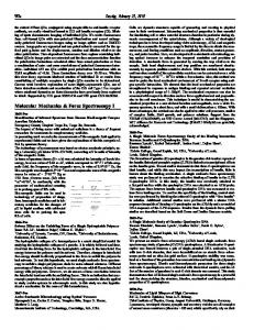
Nanotubes: (Heterogeneity) Single walled nanotube
nanotube bundles
High current flow along tube; z y x
Low current flow perpendicular
Single walled (10,10) nanotube 34
λ (W/cm/K)
32 30 28 26 24 22 20 0
50
100
150
Tube Periodicity (A)
200
250
(10,10) nanotube with vacancies 14
λ (W/cm/K)
12
y = 0.11402 * x^(-0.78849) R= 0.99794
10 8 6 4 2
4
6
8
nv ( per 1000 atoms)
10
12
(10,10) nanotube with (5,7,7,5) defects 35 y = 22.733 * x^(-0.64179) R= 0.99082
λ (W/cm/K)
30 25 20 15 10 0.5
1
1.5
2
nd (per 1000 atoms)
2.5
3
Nanotube Bundles: (Heterogeneity)
Z: 9.5 W/cm/K Graphite // plane: 10. W/cm/K
X,Y: 0.055 W/cm/K z y x
Graphite plane: 0.056 W/cm/K
Friction Models: Static Friction From theory and simulation:
Static Friction Fs: •Commensurate Interface: strongly interaction v=0 when Fx< Fc; i.e. must overcome a threshold force to make motion occur
•Incommensurate Interface: weakly interaction flat, atomically smooth, clean: Fs= 0; with defects, roughness or third body: Fs ≠ 0
Friction Models: Kinetic Friction Kinetic Friction Fk vs. velocity v Fk(v)=Fk(0)+cvβ •Dry Friction: β=0, Coulomb friction kinetic friction has no dependence in the slow sliding limit Observed in experiments for macroscopic system; MD simulation and other atomic-level treatments fail to give this behavior
Viscous Friction: β=1, Stokes friction Kinetic friction is proportional to the velocity It is normally believed that dry friction and static friction are related and if kinetic friction behaves viscous law, there is no static friction.
Constant Force Simulation Constant force simulation to determine the static friction FN z direction movements of top layers are fixed to be zero (one Al layer and one O layer for Al2O3, one Al layer for Al metal)
Fex
f The length of z-direction has been fixed, so the samples are under compression condition. z-direction movements are fixed to be zero External force Fex is applied to the outmost layers
Fex
f
Constant Velocity Simulation Constant velocity simulation to study the kinetic friction z direction movements of top layers are fixed to be zero Vex
For atom n in top layers of top slab: Vn(t1)= Vn(t0)+(Vex-Vcm(t1)) × t Xn(t1)=Xn(t0)+Vn(t1) × t Vcm is the calculated velocity for center of mass, so top slab moves with Vex x and z directions movements are fixed to be zero
f f
Tahir Cagin
Why to talk about mechanics of Nanomaterials? •
•
•
Mechanics of materials is really about the microstructure – Ultimate mechanical properties are on perfect systems – Actual properties observed are something else, (are they?) Properties and especially mechanical properties of small world – Surface to volume ratio (1/L) increases – Properties are determined more and more by this increasing ratio Continuum elasticity is a tool for relating to macro-world, but not the method – Atomistic details are the main player in properties – Applied loads have statistically distributed results – Measured properties depend on small variations in the structure
Nano-mechanics of •
• •
•
Nano-dots, clusters – metallic clusters – dendrimers Nano-wires – nm-size wires of metals, ceramics, and semiconductors Nano-shells – Thin films of metals, – Thin films of Ferro-, piezo- electric materials, semiconductors, – self assembled monolayers of organic films, dendrons Nano-tubes – isolated, bundled single and multiple walled carbon nanotubes, – inorganic and organic (cyclic peptides) nanotubes
Carbon Nanotubes
Carbon Nanotubes with Valence FF
(n1,n2) R2
R1
Stable Forms: Circular / Collapsed? (n,n) -armchair (n,0) - zigzag (2n,n) - chiral
Circular - Collapsed Forms upto R=170A
Stable Forms: Circular to Collapsed transition The cross sectional shape shows a broad transition range at R1 through R2, both circular and collapsed form exist. Below R1, Circular form above R2 collapsed form are stable. The radii of the first transition are: • (n,n) armchair, R1 is between 10.77 A of (16,16) and 11.44 of (17,17). • (2n,n) chiral, R1 is between 10.28 A of (20,10) and 11.31 of (22,11). • (n,0) zigzag, R1 is between 10.49 A of (27,0) and 10.88 of (28,0).
The radii of the second transition are: • (n,n) armchair, R2 is between 29.62 A of (45,45) and 30.30 of (46,46). • (2n,n) chiral, R2 is between 29.82 A of (58,29) and 30.85 of (60,30). • (n,0) zigzag, R2 is between 29.93 A of (77,0) and 30.32 of (78,0).
Zero Strain (axial and radial) Stable Cross Sectional Shapes for (n,m)
Bending modulus of Graphene Basic energetics by approximating the tube as a membrane with a curvature 1/R and bending modulus of κ. Assuming a as the thickness of tube wall, the elastic energy stored in a slab of width L, is given by The per atom energy N is the number of carbon atoms per slab Eο is energy per carbon atom for tubes with 1/R ∼ 0, i.e. flat sheets. Considering the number of carbon atoms per unit area of tube wall
a the spacing between two graphite sheets, 3.335(Å), R0 = 1.410(Å) as the C-C bond distance, κ(n,n) = 963.44 (GPa), κ(n,0) = 911.64 (GPa), and κ(2n,n) = 935.48 (GPa).
Stretching and compressing tubes at cross-over radius
Stretching and compressing tubes at cross-over radius
Structure and mechanical moduli of SWNT Bundles Single Walled CNT Bundles (10,10) armchair lattice parameter a = 16.78 Å, density d = 1.33 (g/cm3). (17,0) zigzag, they are a = 16.52 Å, and d = 1.34 (g/cm3). (12,6) chiral form, they are a = 16.52 Å and d = 1.40 (g/cm3). Young's modulus along the tube axis for triangular-packed SWNTs (using the second derivatives of the potential energy.) Y = 640.30 GPa, armchair Y = 648.43 GPa, zigzag Y = 673.49 GPa, chiral. Normalized to carbon sheet these are within a few % of the graphite bulk value.
Bending Modulus of SWNT from Carbon Nanotori and deformation kinks as deformation sinks
R=19.4 A (2000 atoms) To R=390 A (40,000 atoms)
Strain energy of Tori as a function of 1/R2
Rs > 183 A Circular cross-section smooth torus 183 > Rs > 109 Circular cross section smooth torus, But at RT MD yields dents/creases If MD structure used as input small dents diffuse and merge to make kinks
Emergence of Kinks
Structural Detail of Kinks upon bending
Strain energy of Tori
Kinks/Buckles for Same Rs around Transition
Lowest Energy
R = 109.6 A (10,10,564) with varying # of buckles Lower radii down to 40 A R< 40 A unstable
Torsional Loads
Torsional Loads
Carbon Nanotubes with BO Potentials
(n1,n2) R2
R1
Tensile failure of (10,10) nanotube
Tension waves
(10, 10) Single Wall Nanotube Stretching
Tensile failure of (10,10)-(15,15) double walled nanotube
(10, 10)-(15,15) Double Wall Nanotube Stretching
Bending of (15,15)/(10,10) DWNT 0.8
DWNT (10,10)/(15,15)
0.7
Energy (kcal/mol)
0.6 0.5
BREN
0.4 0.3 0.2
l 3F 2 ∆U = 6 EI
0.1
E=944 GPa
EBOD
0 0
0.2
0.4 Force (nN)
0.6
0.8
1
Plasticity of FCC Nanowires Under High Strain Rate
Apply uniform strain rate: 0.05%/ps, 0.5%/ps, 1%/ps, 2%/ps 5%/ps
for systems as Ni, NiCu and glass former Uniaxial CuAg Stra and NiAu, staring with perfect2nm single crystal.
Infinity along c directio the original unit length i
Stress of NiCu(50%) under different strain rate 10.0
0.05%/ps 0.5%/ps 1%/ps 2%/ps Metallic glass viscosity 5%/ps σ = η dε/dt η=0.8P
Strain Rate: 8.0
stress (GPa)
6.0
4.0
2.0
Fracture 0.0 0.0
0.1
0.2
0.3
0.4
0.5
-2.0 strain
0.6
0.7
0.8
0.9
1.0
Twinning processes at lower strain rate
5
NiCu @ 300K, strain rate = 0.05%/ps
4.5
Accommodate strain by twin formation 7% yield strain Young Modulus is the same after twinning
Stress (GPa)
4 3.5 3 2.5 2 1.5 1 0.5 0 0
0.05
0.1
0.15
0.2
0.25
Strain
Perfect FCCFirst twinsTwins grow
Twin size decreases as strain rate increases
Perfect FCC searching method •
Grain size
250
strain = 40%
200 150 100 50 0 0.5
1
2
strain rate (%/ps)
5
• •
Start from an atoms with the perfect FCC nearest neighbor configuration(ABC packing). Checking the further neighbors. Stop at the boundary where the atoms lost the FCC nearest neighbor structure, and define the number of atoms inside the boundary as the grain size.
Strain rate induced Amorphization Radial distribution function of Ni under slower and faster strain rates •Strain rate = 5%/ps, •Form amorphous, •The second peak on GFR disappeared at strain=15%
•Strain rate = 0.5%/ps, •Twinning started from 7% strain •Kept crystalline structure until 30% strain 7
7 strain = 0
strain = 0
6
strain = 10%
strain = 10%
strain = 20%
5
strain = 15%
5
strain = 30%
g(r)
g(r)
4
strain = 20%
1
4 0
3
3
g(r)
6
2
0.3
0.35
0.4
0.45
0.5
r(nm )
2
2
1
1 0
0 0.2
0.3
0.4
0.5 r (nm)
0.6
0.7
0.8
0.2
0.3
0.4
0.5 r (nm)
0.6
0.7
0.8
350
Elastic constants vs strain
3C66-C44
Strain rate = 5%/ps
300
Shear Moduli recovered due to twinning
250
0.05%/ps
200
Cij (GPa)
Metal glass fully formed C11,C22
150 C33 C12
C22-C23
C66
(C11-C12)/2 (GPa )
40
0.5%/ps 30
5%/ps
20 10 0
100
0
(C11-C12)/2 0 0.2
0.15
Tetragonal shear moduli would vanish at strain = 0.11, which initiated the transition.
C44,C55
0
0.1 strain
C23,C13
50
0.05
0.4
0.6 strain
0.8
1
0.2
• Deformation mechanism beyond defects movements is twinning and amorphization. • Strain rate plays a role similar to temperature. • Disorder causes similar effect in strain rate induced amorphization, that lager size differences lower the strain rate required for amorphization.
Cooling rate strain rate size ration 0.005 0.5 1 2 5
Ni
NiCu 1
1.025 Crystal Crystal Crystal Crystal Crystal Crystal Crystal Amorphous Amorphous Amorphous
NiAu
Amorphous
1.156 Amorphous Amorphous Amorphous Amorphous Amorphous
crystal
Strain rate Size ratio