Sep 17, 2009 - the peak spacing distribution11 and the peak height dis- tributions12 at low ..... sc (r, râ²) get sub- tracted off in the ... This coefficient may in practice be quite large even ..... average vαβ. We note that Eq. (23) is a lower bound.
Interaction matrix element fluctuations in ballistic quantum dots: dynamical effects L. Kaplan1 and Y. Alhassid2
arXiv:0909.3295v1 [cond-mat.mes-hall] 17 Sep 2009
1
Department of Physics, Tulane University, New Orleans, Louisiana 70118, USA 2 Center for Theoretical Physics, Sloane Physics Laboratory, Yale University, New Haven, Connecticut 06520, USA
We study matrix element fluctuations of the two-body screened Coulomb interaction and of the one-body surface charge potential in ballistic quantum dots, comparing behavior in actual chaotic billiards with analytic results previously obtained in a normalized random wave model. We find that the matrix element variances in actual chaotic billiards typically exceed by a factor of 3 or 4 the predictions of the random wave model, for dot sizes commonly used in experiments. We discuss dynamical effects that are responsible for this enhancement. These dynamical effects have an even more striking effect on the covariance, which changes sign when compared with random wave predictions. In billiards that do not display hard chaos, an even larger enhancement of matrix element fluctuations is possible. These enhanced fluctuations have implications for peak spacing statistics and spectral scrambling for quantum dots in the Coulomb blockade regime. PACS numbers: 73.23.Hk, 05.45.Mt, 73.63.Kv, 73.23.-b
I.
INTRODUCTION
The statistical fluctuations of single-particle energies and wave functions of dots whose single-particle dynamics are chaotic may be well approximated by random matrix theory (RMT)1 . The mesoscopic fluctuations of the conductance through open dots that are strongly coupled to leads are then successfully described by RMT2 . In the opposite limit of an almost-isolated dot, the charge is quantized and electron-electron interactions modify the mesoscopic fluctuations of the conductance. The randomness of the single-particle wave functions induces randomness into the interaction matrix elements when the latter are expressed in the basis of the former. These matrix elements can be decomposed into an average and a fluctuating part. The average part of the interaction, when combined with the one-body kinetic energy and a confining potential, leads to the so-called universal Hamiltonian3,4 . This universal Hamiltonian includes a charging energy term and an exchange interaction term that is proportional to the square of the total spin of the dot (an additional Cooper-channel term is repulsive in a quantum dot and can be ignored). The fluctuating part of the interaction is suppressed by the Thouless conductance gT , and in the limit gT → ∞, the dot is completely described by the universal Hamiltonian. The charging energy term leads to charge quantization in a weakly coupled dot, and the conductance peak height distributions in such a dot were derived in Ref. 5 using the RMT statistics of the single-particle wave functions. Qualitative features of these peak height distributions as well as the parametric peak height correlation and the weak localization effect as a function of magnetic field6,7 were confirmed in experiments8,9,10 . Remaining discrepancies between theory and experiments regarding the temperature dependence of the width of the peak spacing distribution11 and the peak height distributions12 at low temperatures were explained by the inclusion of the exchange interaction term of the univer-
sal Hamiltonian13,14 . However, not all observed features of the peak spacing distribution can be explained by the exchange interaction alone. At low temperatures, the spacing is given by the second-order difference of the ground-state energy versus particle number. When only charging energy is present, the peak spacing distribution is expected to be bimodal because of spin effects. The exchange interaction (with realistic values of the exchange coupling constant in quantum dots) reduces this bimodality but cannot explain its absence in the experiments11,15,16,17 . It is then necessary to consider the effect of the fluctuating part of the interaction beyond the universal Hamiltonian. In the Hartree-Fock-Koopmans approach, the peak spacing can be expressed in terms of certain interaction matrix elements, and sufficiently large fluctuations of such matrix elements18 might explain the absence of bimodality in the peak spacing distribution. It is therefore of interest to make accurate estimates of interaction matrix element fluctuations in chaotic dots. These fluctuations are determined by single-particle wave function correlations. In a diffusive dot, such correlations are well understood and lead to an O(∆/gT ) standard deviation in the interaction matrix elements19,20 , where ∆ is the mean single-particle level spacing. Peak spacing fluctuations are also affected by a one-body surface charge potential induced by the accumulation of charge on the surface of the finite dot19 . Matrix element fluctuations of the two-body interaction and one-body surface charge potential are also important for determining the statistical scrambling of the Hartree-Fock energy levels and wave functions as electrons are added to the dot21,22 . Wave function correlations and interaction matrix elements fluctuations in a ballistic dot are less understood. In Ref. 23 we used a normalized random wave model to obtain analytic expressions for interaction matrix element variances and covariances in the regime of large Thouless conductance gT for a ballistic two-dimensional dot. In such a dot, gT ∼ kL, where k is the Fermi wave
2 number and L is the linear size of the dot (defined more precisely √ as the square root of the dot’s area). Since kL ∼ N where N is the number of electrons in the dot, the kL ≫ 1 limit in which the random wave model is expected to hold is also the limit of many electrons in the dot. In the present work, we systematically investigate matrix element fluctuations in real chaotic billiards, for 30 ≤ kL ≤ 70, corresponding roughly to the parameter range relevant for experiments (∼ 150 − 800 electrons in the dot). We show that fluctuations can be significantly enhanced due to dynamical effects, e.g., the variance may be enhanced by a factor of 3 or 4. Such enhancement can help in explaining the peak spacing distribution measured in the chaotic dots of Ref.11 . On the other hand, the typical fluctuations of matrix elements in chaotic dots cannot explain the even broader peak spacing distributions in the experiment of Ref. 17. The small dots used in the latter experiment are probably non-chaotic (top gates were used), and this has motivated us to study fluctuations beyond the chaotic regime. We show that a large (i.e., order of magnitude) enhancement of the fluctuations is possible in non-chaotic billiards. The outline of this paper is as follows. In Sec. II, we introduce the modified quarter-stadium billiard as a convenient model for investigating matrix element fluctuations in chaotic systems. In Section III we consider matrix elements of the two-body screened Coulomb interaction, and find strong enhancement of the fluctuations in comparison with random wave predictions. Semiclassical corrections due to bounces from the dot’s boundaries lead to an increase in the fluctuations, but do not correctly predict the scaling with kL in the experimentally relevant range. Insight into the underlying mechanism of fluctuation enhancement is obtained by studying a quantum map model, which is described in the Appendix. An important conclusion is that the expansion in 1/kL, while asymptotically correct, can be problematic in quantifying matrix element fluctuation in the regime relevant to experiments. In Sec. IV we extend our investigation to one-body matrix elements associated with the surface charge potential, and find similar fluctuation enhancements. Going beyond the variance, we examine the full matrix element distributions in Sec. V, and observe deviations from a Gaussian shape that are even stronger than the deviations found in the random wave model23 . In Sec. VI we study systems beyond the chaotic regime: billiards dominated by marginally-stable bouncing-ball modes and billiards with mixed dynamics (i.e., partly regular and partly chaotic). Finally, in Sec. VII we briefly discuss some implications of the present work for the quantitative understanding of spectral scrambling and peak spacing statistics for quantum dots in the Coulomb blockade regime.
II.
CHAOTIC BILLIARDS
Here we investigate how dynamical effects modify the fluctuations of interaction matrix elements beyond our findings in the random wave model23 . Here and in Sections III – V we treat exclusively geometries displaying hard chaos. [Systems with stable or marginally stable classical trajectories will be considered in Sec. VI.] To this end, we will use a chaotic system shown in Fig. 1 – a modified quarter-stadium billiard geometry24 , where the quarter-circle has radius R and the straight edge of length aR has been replaced by a parabolic bump to eliminate bouncing-ball modes. Algebraically, the billiard shape is defined by � � x2 0 ≤ y/R ≤ 1 − s 1 − 2 2 , 0 ≤ x/R ≤ a a R p 0 ≤ y/R ≤ 1 − (x/R − a)2 , a ≤ x/R ≤ a + 1 , (1)
where R is the radius of the quarter-circle, and a and s are free dimensionless parameters.
s r2 r1 1-s
1
a
FIG. 1: A modified quarter-stadium geometry with parameters a and s is used to illustrate dynamical effects on matrix element fluctuations. In the figure, we set the quarter-circle radius R = 1. The random wave contribution to the wave function intensity correlator C(r1 , r2 ) is schematically indicated by a dashed line, and a typical dynamical contribution by a dotted line.
We use a quarter-stadium instead of a full stadium shape in order to remove symmetry effects. This system has been verified numerically to be fully chaotic for the range of parameters used. Variation of the bump size s allows us to check the sensitivity of the results to details of the billiard geometry while maintaining the chaotic character of the classical dynamics. Furthermore, by varying the parameter a, we can control the degree of classical chaos. The degree of chaos can be characterized for example by the Lyapunov exponent λ, defined as the rate of divergence at long times of generic infinitesimally separated trajectories, |r(t)−r′ (t)| ∼ |r−r′ |eλt as |r−r′ | → 0
3 and then t → ∞. For a = 1.00 and 0.1 ≤ s ≤ 0.2, the exponent λ takes values 0.69 ≤ λTB ≤ 0.74 (here TB = mL/¯hk is a typical time scale associated with one bounce in the billiard). When a = 0.25, 0.55 ≤ λTB ≤ 0.56 in the same range of s, indicating that the system is somewhat less chaotic for the smaller value of a. Other measures of the degree of chaoticity are possible and may be more relevant to the problem of matrix element fluctuations, as we will argue below. In particular, we may consider the rate λ∗ of long-time decay of classical corre2 lations, f (q, p)f (q(t), p(t)) − f (q, p) ∼ e−λ∗ t as t → ∞, where f (q, p) is a typical function defined over the classical phase space and the average is over an energy hypersurface25 . Numerically, we find 0.15 ≤ λ∗ TB ≤ 0.20 for a = 1 and 0.095 ≤ λ∗ TB ≤ 0.13 for a = 0.25, for the same range of bump sizes s as above, again indicating a less rapid approach to ergodicity in the a = 0.25 geometry. An important consideration in the investigation of dynamical systems, as opposed to random wave models, is the presence of boundary conditions. Boundary conditions lead to Friedel oscillations in the average wave function intensity at distances O(1/k) from a billiard boundary. The effect of such oscillations has recently been considered in Refs. 26. The choice of boundary conditions, e.g., Neumann or Dirichlet, will also be seen to have significant effects on matrix element fluctuations, particularly on the fluctuations of one-body matrix elements. Numerical wave functions for several values of the billiard parameters a, s and in various energy ranges have been calculated using a variation of the plane wave method27 . At each wave number k, a basis consisting of plane waves supplemented by a set of Y0 Bessel functions centered a fraction of a wavelength outside the boundary is used; the size of the basis scales linearly with k. Singular value decomposition finds at each k the linear combination that minimizes the integrated squared deviation along the boundary from the selected boundary condition (Dirichlet or Neumann). Finally, minima of this deviation as a function of k indicate the correct eigenvalues of the system. Tests of the method include stability with respect to changes in the basis size and comparison of the resulting density of states with the Weyl formula. Statistics are collected by averaging over an energy window. A straightforward estimate shows that such averaging is sufficient to give good results for matrix element variances, i.e., the ratio of signal to statistical noise grows with increasing kL. For all numerical results that follow, we use energy windows of constant momentum width ∆k L = 10, e.g., the data point kL = 30 uses all wave functions within the window 25 ≤ kL ≤ 35. The Weyl formula for the density of states in two dimensions implies that the number of wave functions in such a window grows linearly with kL.
III. A.
TWO-BODY MATRIX ELEMENTS
Fluctuation of diagonal matrix elements vαβ
We first study the variance of the diagonal two-body interaction matrix elements vαβ ≡ vαβ;αβ , associated with a pair of electrons in distinct orbitals α 6= β interacting via the screened Coulomb force. Since the screening length of the Coulomb interaction in large 2D quantum dots is much smaller than the dot size, the interaction may be modeled as a contact interaction v(r, r′ ) = ∆ V δ(r − r′ ), where V = L2 is the dot’s area, and the single-particle mean level spacing ∆ serves to set the energy scale28,29 . We then have Z vαβ = ∆ V dr |ψα (r)|2 |ψβ (r)|2 , (2) V
where the single-electron wave functions ψ obey the usual R normalization condition V dr |ψ(r)|2 = 1. To leading order in 1/gT ∼ 1/kL, the variance is then given by21,23 : � � Z Z ∆2 2 = ∆2 V 2 , (3) δvαβ dr dr′ C 2 (r, r′ ) + O (kL)3 V V where C(r, r′ ) = |ψ(r)|2 |ψ(r′ )|2 − |ψ(r)|2 |ψ(r′ )|2
(4)
is the intensity correlator of a single-electron wave function at points r and r′ . Assuming C(r, r′ ) is described by the normalized random-wave model (i.e., the singleelectron wave functions are normalized as above with no boundary conditions), one obtains � �2 � � 2 ln kL + bg ∆2 23 2 δvαβ = ∆ , (5) +O π β (kL)2 (kL)3 where β = 1, 2 corresponds to the presence or absence of time reversal invariance (i.e., the absence or presence of an external magnetic field), while bg is a dimensionless coefficient that weakly depends on the dot geometry23 . We now evaluate the variance of vαβ versus kL using “exact” (numerically evaluated) real wave functions in actual chaotic billiards. Typical results are shown in Fig. 2, where we note the large enhancement of the billiard results over the random wave model (dotted line). To understand this enhancement, we compare the ex2 with the first term on the act numerical results for δvαβ right hand side of Eq. (3), in which C(r, r′ ) is taken to be the single-wave-function correlator Cbill (r, r′ ) calculated numerically for the appropriate billiard system. The discrepancy is immediately reduced to a ∼ 5 − 10% level, which is comparable to the O((kL)−3 ) higher-order correction expected and observed in the random wave model. Thus, the large enhancement of vαβ fluctuations over the random wave prediction is not due to higher-order terms in Eq. (3), but instead can be traced directly to a dynamical enhancement in the intensity correlator Cbill (r, r′ ) over the random-wave correlator.
4 while the Green’s function is given by the Gutzwiller formula32 X 1 |Dj |1/2 eiSj /¯h−iµj π/2 . (9) G(r, r′ , E) = 1/2 i¯h(2πi¯h) j
5×10⁻²
(δvαβ)2
2×10⁻² 1×10⁻² 5×10⁻³
2×10⁻² 1×10⁻²
2×10⁻³ 1×10⁻³
30
50
30
70
40
50
60
70
kL
FIG. 2: The variance of vαβ versus kL (on a log-linear scale) for modified quarter-stadium billiards with Neumann boundary conditions. The solid line is for a = 0.25, while the dashed line is for a = 1.00. In both cases, the results are averaged over two values of the bump size: s = 0.1 and 0.2. Dotted line: analytic random wave prediction, Eq. (5). Inset: the numerical result for a = 0.25 with the leading logarithmic term of Eq. (5) subtracted (solid line) appears to fall off as (kL)−1.15 (dashed line). The analytically expected subleading behavior (kL)−2 is indicated by a dotted line for comparison.
We next estimate the dynamical enhancement of the intensity correlator (as compared with a random wave model) in a semiclassical approach. The random wave correlator Crw (r, r′ ) may be interpreted semiclassically as arising from straight-line free propagation20 indicated by the dashed line in Fig. 1. As discussed by Hortikar and Srednicki30 and more recently by Urbina and Richter31 , additional contributions to the correlator can be associated with trajectories that bounce off the boundary n times on their way from r to r′ , such as the one indicated by a dotted line in Fig. 1. To find these contributions, we start from the dynamical correlator for wave function amplitudes, which may be written as30,31 ∗
G (r, r′ , E) − G(r′ , r, E) ψ ∗ (r)ψ(r′ ) = , 2πi ρ(E)
(6)
where G is the ensemble-averaged part of the retarded P ψα∗ (r)ψα (r′ ) Green’s function G(r, r′ , E) = α E−E , and ρ(E) α +iǫ is the smooth part of the density of states ρ(E) = P δ(E − E ). Using Eqs. (4), (6), the dynamical inα α tensity correlator is given by Cbill (r, r′ ) =
2 ∗ |G(r′ , r, E)−G (r, r′ , E)|2 /4π 2 ρ2 (E) .(7) β
Semiclassically, the smooth density of states is given to leading order by the Weyl formula in two dimensions ρ(E) = mL2 /2π¯ h2 ,
(8)
The sum in (9) is over classical trajectories j connecting r to r′ at energy E, Sj is the action along the trajectory j, µj is the corresponding Maslov index, and Dj is a classical focusing factor that scales as m2 /pLj (where Lj is the length of the trajectory). For the straight-line trajectory, |Dj | = m2 /p|r − r′ |. Inserting the semiclassical expressions (8) and (9) into Eq. (6), we obtain i 1 h J0 (k|r − r′ |) + h(r, r′ )(kL)−1/2 , ψ ∗ (r)ψ(r′ ) = V (10) where the Bessel function arises from the straight-line path, and h(r, r′ ) is a sum over all other trajectories: h(r, r′ ) =
′ X
hj (r, r′ )
j
1 � � ′ X 2pLDj 2 Sj (2µj + 1)π = . (11) πm2 cos ¯h − 4 j
For typical point pairs (r, r′ ) separated by a distance of order L, the function h(r, r′ ) is order unity in kL, and the contributions to the correlator from the straight line path and from other paths are both O((kL)−1/2 ). For pairs (r, r′ ) separated by a bouncing path of length Lj /L ≤ ǫ ≪ 1, h(r, r′ ) ∼ ǫ−1/2 . However, the fraction of such pairs is O(ǫ3 ) and their contribution to the variance and other moments of matrix element distributions is negligible. The intensity correlator in the semiclasssical approximation becomes 1 2� 2 Csc (r, r′ ) = J (k|r − r′ |) + h2 (r, r′ )(kL)−1 V2β 0 + 2J0 (k|r − r′ |)h(r, r′ )(kL)−1/2 ] ,
(12)
where the first (random wave) term is associated with the straight-line path, and the remaining terms constitute semiclassical corrections. Similarly to the random wave correlator23,33,34 , Csc (r, r′ ) must be corrected to take into account individual wave function normalization. In analogy with Refs. 23,33 we have, to leading order in 1/kL, Z Z 1 dra drb Csc (ra , rb ) C˜sc (r, r′ ) = Csc (r, r′ ) + 2 V Z ZV V 1 1 − dra Csc (r, ra ) − dra Csc (ra , r′ ) . (13) V V V V Substituting C˜sc for C in (3), we find � �2 � � 2 (ln kL + bg ) + bsc ∆2 2 = ∆2 3 , + O δvαβ π β (kL)2 (kL)3 (14)
5 where bsc is a classical constant that in practice must be determined numerically by performing the integral in Eq. (3). As noted above, the random wave and semiclassical contributions to Csc (r, r′ ) are of the same order except for |r − r′ | ≪ L; it is these short-distance pairs that result in a logarithmic enhancement of the randomwave term. We may easily estimate the dependence of bsc on the degree of chaoticity of the dynamical system by invoking a diagonal approximation, in which the intensity correlator Csc (r, r′ ) of Eq. (12) is averaged over classically small regions surrounding r and r′ . Noting that Eq. (11) gives h(r, r′ ) as a sum of oscillatory terms with quasi-random phases, such averaging leads to dg (r, r′ ) = Csc
′ � 1 2� 2 1 X 2 ′ hj (r, r′ ) , (15) J (k|r−r |)+ 0 2 V β kL j
P′ where j h2j (r, r′ ) corresponds to the total classical probability of traveling from a neighborhood of r to a neighborhood of r′ via paths j other than the straight-line path. Naively, the average semiclassical correction to the intensity correlator appears to increase as we include longer trajectories. However, let us organize the trajectories by number of bounces n or by time t ∼ nTB , where TB is a typical time for one bounce in the billiard. Trajectories at times t that are significantly longer than the classical correlation decay time λ−1 ∗ contribute only dg a constant, independent of r and r′ , to Csc (r, r′ ). This is because a classical cloud of trajectories centered near r becomes approximately equidistributed over the entire billiard when eλ∗ t ≫ 1, for any initial point r. Such dg position-independent contributions to Csc (r, r′ ) get subtracted off in the normalization procedure (13). Thus, the typical size of Csc (r, r′ ) is determined by trajectories j having no more than nmax ≈ (λ∗ TB )−1 bounces. Furthermore, as a function of t, the number of classical trajectories typically grows as eλt , while the focusing factor for each trajectory j falls off as |Dj | ∼ e−λt , where λ is the Lyapunov exponent defined earlier. Thus, all n-bounce trajectories combine to form a contribution to Eq. (15) whose order is roughly n-independent for n < nmax . Summing over n up to nmax , where nmax is large, we find � � �� 1 2 nmax b1 dg Csc (r, r′ ) = 2 J02 (k|r − r′ |) + O , V β kL (16) where b1 characterizes the size of the semiclassical contribution from one-bounce trajectories. Going beyond the diagonal approximation is necessary to evaluate properly the integral in Eq. (3), but the scaling is unaffected. Comparing Eqs. (3), (14), and (16), we obtain an estimate for the coefficient bsc in Eq. (14) describing the semiclassical correction to the random wave model � �2 b1 2 2 bsc ∼ nmax b1 ∼ . (17) λ∗ TB
This estimate confirms our intuition that semiclassical corrections to the random wave approximation become increasingly important as we consider billiards with a very long ergodic time λ−1 ∗ . Alternatively, the scaling (17) may be obtained by noting that when classical correlations persist on a time scale λ−1 that is much longer than the one-bounce time TB , ∗ then the effective dimensionless Thouless conductance is reduced to gT ∼ (λ∗ TB )kL. Now a typical chaotic wave function ψα (r) may be written as a superposition of O(gT ) non-ergodic basis states ηi (r). Since the correlator ηi∗ (r)ηi (r′ ) for each non-ergodic basis state ηi is of order V −1 , we easily see that ψα∗ (r)ψα (r′ ) takes typical −1/2 values of order V −1 gT . The wave function intensity ′ correlator Csc (r, r ) scales as the square of the amplitude correlator, or as V −2 gT−1 for typical pairs (r, r′ ), yielding a lower bound 2 ∼ δvαβ
∆2 ∆2 ∼ 2 gT (λ∗ TB kL)2
(18)
for the integral (3), consistent with Eqs. (14) and (17). For “generic” chaotic systems, the correlation decay time λ−1 is of the same order as the one-bounce time ∗ TB , and the above scaling arguments for λ∗ TB ≪ 1 are not applicable. Instead, only the first few bounces may contribute in practice to the semiclassical correlator, but these must be summed up numerically to obtain the semiclassical coefficient bsc . This coefficient may in practice be quite large even for generic chaotic systems (e.g., the modified stadium billiard) and grows as the system becomes less chaotic. Qualitatively, the above discussion is consistent with our billiard results shown in Fig. 2, as fluctuations are observed to be consistently larger for the less chaotic a = 0.25 billiard, as compared with the a = 1.00 billiard. We note that both billiards are “generic”, in the sense that they are not fine-tuned to obtain an anomalously long time scale λ−1 ∗ . We also note that varying the bump size s has a very weak effect on the matrix element statistics (as long as s is large enough to destroy the bouncing-ball modes) and serves instead to provide an estimate of the statistical uncertainty in our results. For the modified quarter-stadium billiard, we have found that adding one-bounce effects to the random wave correlator increases the predicted vαβ variance by ∼ 30 – 40% in the energy range of interest, a significant change but not nearly sufficient to explain the full factor of 3 – 5 enhancement observed in Fig. 3 for the a = 0.25 billiards (solid lines). Indeed, a close look at the data suggests that the numerical results cannot be explained fully by semiclassical arguments, no matter how many bounces are included in the analysis. The semiclassical correction to the variance in Eq. (14) is manifestly O(1/(kL)2 ). However, the inset in Fig. 2 clearly shows that the dynamical contribution to the variance with kL is not consistent with Eq. (14) but instead appears to follow a much slower power law ∼ 1/(kL)−1.15 . This may
12
10-1
10
10-2
8
10-3
6
S
(δv)2 / (δvrandom)2
6
10-4 4 10-5
2 0 30
50
70
140
kL
10-6
10
100
1000 N
FIG. 3: The enhancement of the variance of vαβ (solid line), vαα (dashed line) and vαβγδ (dotted line) over the corresponding random wave predictions is shown for a = 0.25 billiards. [For vαβ , the random wave prediction is given by Eq. (5), and analogous expressions for the other matrix elements may be found in Ref. 23.] In each case, the data is averaged over bump sizes s = 0.1 and 0.2.
FIG. 4: The two-body matrix element variance S for a quantum map, Eq. (A6) in the Appendix, as a function of the Hilbert space dimension N . From top to bottom, the three solid lines represent data for dominant orbit stability exponent λ0 = 0.25, 0.50, 1.00. The three dashed lines indicate the asymptotic 1/N 2 behavior for each case in the semiclassical regime of large N .
be seen also in Fig. 3 (solid line), where the enhancement over the random wave prediction grows instead of diminishing with increasing kL. We believe this anomalous behavior results from a combination of two related factors: the dynamical enhancement, discussed above, of the bsc coefficient due to a finite correlation time scale λ−1 ∗ in an actual dynamical system, and the consequent saturation of the 1/(kL)2 behavior at moderate (< ∼ 100) values of kL. As the classical system becomes less unstable and the correlation time λ−1 ∗ increases, bsc also increases in accordance with Eq. (17), leading to greatly enhanced matrix element variance at very large values of kL (14). Because the variance is bounded above independent of kL, the (kL)−2 growth in the variance necessarily breaks down for smaller values of kL. This small-kL saturation sets in at ever larger values of kL as the system becomes less unstable and λ−1 ∗ becomes larger. Alternatively, one may note that the natural expansion parameter for interaction matrix element fluctuations in a dynamical system is not (kL)−1 but rather the inverse Thouless conductance gT−1 ∼ (λ∗ TB kL)−1 , and the semiclassical contribution with prefactor bsc in Eq. (14) is the leading O(gT−2 ) effect in such an expansion. Terms of third and higher order in gT−1 , although formally subleading and not included in a semiclassical calculation, become quantitatively as large as the leading O(gT−2 ) term when gT falls below some characteristic value. Furthermore, if one considers chaotic billiards with a long correlation decay time λ−1 ∗ , the importance of formally subleading terms in the gT−1 expansion will extend to quite large values of kL. The above assertions are explicitly confirmed for a
quantum map model, described in detail in the Appendix, which has scaling behavior analogous to that of a two-dimensional billiard, with the number of states N = 2π/¯h playing the role of semiclassical parameter kL = pL/¯h in the billiard35,36 . As in the billiard, a free parameter in the definition of the map allows for control of the classical correlation decay time λ−1 ∗ . A key difference between the two-dimensional billiard and the map model is that the map lacks a logarithmic random wave contribution to the variance. We see in Fig. 4 that the expected N −2 behavior of the variance is observed at sufficiently large N , for all three families of quantum maps considered. Furthermore, the prefactor multiplying N −2 in each case agrees with that obtained from a semiclassical calculation, and as expected this prefactor grows with increasing classical correlation time λ−1 ∗ (corresponding to a decrease in the chaoticity of the system). We also see in Fig. 4 that even for a “typical” chaotic system (i.e., λ∗ TB ∼ 1), strong deviations from the 1/N 2 law appear already below N ≈ 80. Such deviations extend to even larger N for chaotic systems with slower classical correlation decay. This suggests that the largeN or large-kL expansion, though theoretically appealing and asymptotically correct, is problematic in describing the quantitative behavior of interaction matrix element fluctuations for real chaotic systems in the physically interesting energy range. The above numerical calculations were all performed in the presence of time reversal symmetry (β = 1). From Eq. (14) we see that when time reversal symmetry is broken (β = 2), both the random wave contribution to the matrix element variance (the term proportional to ln kL + bg ) and the semiclassical contribution (the term
7 proportional to bsc ) are suppressed by the same factor of 4. Thus, the dynamical enhancement factor for a given dot geometry is necessarily β-independent in the semiclassical limit kL ≫ 1. However, the saturation effect, which tends to suppress the enhancement as kL is reduced, will be less important when β = 2, since the variance is smaller in this case. Thus, at any finite value of kL, the dynamical enhancement in the variance over the random wave model will be greater when time reversal symmetry is broken, and one may expect enhancements somewhat larger than those shown in Fig. 3. This result has been confirmed in the quantum map model.
rounding a periodic orbit. Comparing with the integral expression (3) for the variance, we see that periodic orbits asymptotically contribute to the variance only at order 1/(kL)3 , compared to the O(1/(kL)2 ) semiclassical effect associated with generic (non-periodic) classical trajectories (14). Thus, the relative importance of periodic orbit effects on matrix element fluctuations is a finite-kL (or finite-¯ h) phenomenon, which cannot explain the quantitative scaling behavior of the variance with kL, and which is expected to become irrelevant in the asymptotic kL → ∞ limit. C.
B.
Matrix element covariance δvαβ δvαγ
Fluctuation of vαα and vαβγδ
2 of doubleWe have similarly studied the variance δvαα diagonal interaction matrix elements and the variance 2 δvαβγδ of off-diagonal interaction matrix elements for actual chaotic billiards. Once again, the random wave predictions23 must be used as the baseline for comparison. In Fig. 3, we show the enhancement factor for these matrix element variances, together with the corresponding 2 discussed previously. data for δvαβ In the range 30 ≤ kL ≤ 70 most relevant to experi2 over the ranment, we observe an enhancement in δvαα dom wave prediction that is similar to the enhancement 2 in the same energy range. In both cases, the enin δvαβ hancement factor continues to grow, instead of approaching unity, at increasing kL. This latter fact strongly suggests that even at kL = 140, we are still far from the asymptotic regime of large gT , where matrix element fluctuations would be adequately described by a random wave picture supplemented by semiclassical corrections. The enhancement at large kL is particularly dramatic 2 in the case of δvαα fluctuations. On the other hand, the variance of off-diagonal matrix elements vαβγδ is enhanced over the random wave prediction by at most 10%, over the entire energy range considered. This is consistent with the reasonable expectation that dynamical effects lead to particularly strong deviations from random wave behavior in a modest fraction of the total set of single-particle states, such as those associated with particularly strong scarring on unstable periodic orbits37 . Such deviations lead to a significant tail in the vαα distribution, but have a minimal effect on the distribution of off-diagonal matrix elements, since it is unlikely for all four wave functions ψα , ψβ ψγ , and ψδ to be strongly scarred or antiscarred on the same orbit. Indeed, inspection of wave functions ψα associated with anomalously high double-diagonal matrix elements vαα shows that these wave functions have disproportionately high intensity on average near the dominant horizontal bounce periodic orbit, which follows the lower edge of the billiard in Fig. 1. We note, however, that asymptotic scar theory in the kL → ∞ limit predicts O(1/(kL)) corrections to the intensity correlation function in position space and only in a region of size O(1/(kL)1/2 ) sur-
The normalized random wave model has been shown to produce a covariance δvαβ δvαγ that is always negative, has size ∼ ∆2 ln kL/(kL)3 for small ω = Eβ − Eω , and falls off as (ω/ET )−2 ∼ (δkL)−2 for ω ≫ ET , where ET is the ballistic Thouless energy23 . However, in a diffusive dot, the same matrix element covariance is found to be a positive constant ∝ ∆2 /gT3 (where gT is the diffusive Thouless conductance) for energy separations ω much smaller than the diffusive Thouless energy Ec . This diffusive covariance falls off for ω ≫ Ec but remains positive as long as ω ≪ ¯h/τ , where τ is the mean free time21 . An interesting issue is then the sign of the covariance in an actual chaotic system. First we note the sum rule23 X X δvαβ δvαγ = − (δvαβ )2 . (19) β6=γ
β
This sum rule is quite general and holds for either a ballistic or a diffusive dot as long as a completeness relation is satisfied within an energy window in which the states β and γ reside. The average covariance must therefore be negative when averaged over all states β and γ within such an energy window. The size of the energy window in each case must be at least of size ¯h multiplied by the inverse time scale of first recurrences. In a ballistic system this implies an energy window of size at least E0 = h ¯ /TB , where TB is the one-bounce time. In a diffusive system, the completeness relation requires energy scales larger than E0 = h ¯ /τ , where τ is the mean free time, and thus the positive sign of the diffusive covariance at energy separations ω ≪ ¯h/τ does not contradict the sum rule (19). In actual chaotic billiards, it is in principle possible to find positive covariance at energy scales ω ≪ E0 , as long as the covariance is sufficiently negative for ω ∼ E0 to produce a negative average covariance over the full energy window that is consistent with the sum rule (19). Such positive covariance can result from scars since ψβ and ψγ will typically be scarred or antiscarred along the same orbits when ω = Eβ − Eγ is small. The scar contribution to the covariance for small ω is O(1/(kL)3 ) (i.e., of the same order as the scar contribution to the variance) and is formally subleading compared with the negative O(ln kL/(kL)3 ) random wave contribution. How-
8
(δvαβ) (δvαγ) / (δvαβ)2
0.2 0.1
0.12 (δvαβ) (δvαγ) / (δvαβ)2
ever, within the range of kL values relevant to experiments, the scar contribution can dominate and lead to a positive covariance for nearby single-particle wave functions.
0.08
0.04
0
-0.04
0
0.1
1 ω / E0
-0.1 -0.2 0
1
2
3
ω / E0
FIG. 5: The covariance δvαβ δvαγ is computed as a function of energy separation ω = Eβ − Eγ for an ensemble of ballistic discrete-time maps, described in the Appendix, Eqs. (A9) and (A10). Here E0 = ¯ h/TB , where TB is the one-bounce time. The system size N is 128, and A = 0. The dotted line indicates the negative average covariance implied by the sum rule (19).
Unfortunately, it is not practical to calculate the matrix element covariance in a real billiard, since the number of wave functions that can be averaged over is not sufficient to obtain a signal larger than the statistical noise. We instead obtain good statistics for the covariance in a ballistic discrete map model, introduced previously in the discussion of the variance, and described in detail in the Appendix. In such discrete maps, the matrix element variance or covariance contains no logarithmic terms. For generic chaotic ballistic systems (i.e., Lyapunov time of the same order as the one-step time), we find that the covariance is O(N −3 ) ∼ O((kL)−3 ) and positive for ω ≪ E0 = h ¯ /TB , but becomes negative at ω ∼ E0 , in contrast with the random wave prediction of an always negative covariance. A typical example for N = 128 is shown in Fig. 5. Here discreteness of time implies energy periodicity with period 2πE0 = 2π¯h/TB , and thus a maximum energy separation ω = πE0 . In Fig. 5, the dotted line indicates the negative average covariance over the entire energy window of size 2πE0 , as required by the sum rule (19). It is interesting to compare with the covariance in an ensemble of two-dimensional diffusive discrete maps38 . Typical data is shown in Fig. 6 for an ensemble of diffusive maps on a 32x32 lattice, with Thouless conductance gT = 12 (solid curve) and gT = 24 (dashed curve). The theory predicts a variance scaling as 1/gT2 and a covari2 should scale as ance scaling as 1/gT3 , so δvαβ δvαγ /δvαβ 1/gT in the gT → ∞ limit. Just as in the ballistic case,
FIG. 6: The covariance δvαβ δvαγ is computed as a function of energy separation ω = Eβ − Eγ for an ensemble of diffusive discrete-time maps on a 32x32 lattice38 . The solid curve corresponds to Thouless conductance gT = 12 (Ec /E0 = 0.074) and the dashed curve corresponds to gT = 24 (Ec /E0 = 0.147). Here E0 = ¯ h/τ , where τ is the mean free time. The value ω = Ec , below which the covariance is expected to approach a constant positive value, is indicated by a circle in each case. The dotted line indicates the negative average covariance implied by the sum rule (19).
the covariance is positive for small separations ω and becomes negative when ω ∼ E0 . The average covariance over a maximal energy window of size 2πE0 is again negative, as predicted by the sum rule (19) and indicated by a dotted line. IV.
ONE-BODY MATRIX ELEMENTS
When an electron is added to the finite dot, charge accumulates on the surface and its effect can be described by a one-body potential energy V(r). The diagonal matrix elements of V(r) are given by vα ≡ Vαα = R 2 dr |ψ α (r)| V(r), and the variance of these one-body V matrix elements may be computed as Z Z dr dr′ V(r)C(r, r′ )V(r′ ) . (20) δvα2 = V
V
Dynamical enhancement of one-body matrix element fluctuations may be studied similarly to the analysis of two-body matrix element fluctuations presented in Sec. III. The leading semiclassical contribution to the variance is obtained by substituting the normalized semidg classical intensity correlator Csc [see Eq. (16)] for C(r, r′ ) in Eq. (20). We immediately obtain � � ∆2 cg + csc ∆2 2 , (21) +O δvα = β kL (kL)2 where cg is a geometry-dependent dimensionless coefficient arising already in the random wave model23 , while
9
5×10⁻³
4.5 4 (δvα)2 / (δvα,random)2
csc ∼ (λ∗ TB )−1 is associated with the classical dynamics. We note that the asymptotic power-law behavior of the variance is unchanged from the random wave model, and the variance is enhanced only by a kL-independent constant.
3.5 3 2.5 2
(δvα)2
1.5 1
2×10⁻³
30
40
50
60
70
kL 1×10⁻³
5×10⁻⁴
FIG. 8: Enhancement factor of the vα variance over the random wave prediction is plotted for modified quarter-stadium billiards with Neumann boundary conditions, averaged over s = 0.1 and 0.2. Solid line: a = 0.25; dashed line: a = 1.00. 30
40
50
60
70
kL
V.
FIG. 7: The variance of the one-body diagonal matrix element vα for modified quarter-stadium billiards (a = 0.25; averaged over s = 0.1 and s = 0.2) is plotted as a function of semiclassical parameter kL. Solid line: Neumann boundary conditions. Dashed line: Dirichlet boundary conditions on curved boundaries, and Neumann boundary conditions elsewhere. Dotted line: Analytic prediction for the random wave model (given by Eq. (21), including only the cg term).
Numerical data for δvα2 in modified quarter-stadium billiards is presented in Fig. 7, and compared with random wave results. The ratio of the actual variance to the random wave prediction is shown in Fig. 8. Clearly this ratio is not constant but rather grows with kL (as was also the case with the vαβ variance), indicating once again that at kL ≈ 70 we have not yet reached the asymptotic large-kL regime where semiclassical expressions become applicable. The same can be observed by comparing data for Neumann and Dirichlet boundary conditions in Fig. 7. Since Dirichlet wave functions decay to zero at distances less than 1/k from a boundary, where the surface potential is especially strong, we expect larger matrix element fluctuations for the Neumann boundary condition data, qualitatively consistent with the results in the figure. However, the fraction of points r so close to the boundary is O(1/kL), while the surface potential V(r) is only enhanced by O((kL)1/2 ) there, so the boundary condition effect is formally subleading. Nevertheless, we clearly see from the figure that in the energy range of experimental interest, the boundary condition effect is of size comparable both to the dynamical enhancement and to the baseline random wave prediction for the variance.
MATRIX ELEMENT DISTRIBUTIONS
Just as was done previously for the random wave model23 , we can go beyond the variance to investigate higher moments of the matrix element distribution for actual chaotic systems. A typical distribution for diagonal two-body matrix elements vαβ in a modified quarterstadium billiard with a = 0.25 and s = 0.1 is shown in Fig. 9. Since the approach to Gaussian behavior is already very slow in the case of random waves, it is not surprising to find even stronger deviations from a Gaussian shape for matrix elements in real chaotic systems at the same energies. Thus, for modified quarter-stadium billiards with a = 1, the skewness γ1 of the vαβ distribution grows from 1.95 at kL = 70 to 2.72 at kL = 140, while the skewness for the same geometry in the random wave model drops slightly from 1.21 to 1.09. Similarly, the excess kurtosis γ2 increases from 8.3 at kL = 70 to 20.9 at kL = 140, while dropping from 3.7 to 3.3 in the random wave model. Similar behavior is obtained for other matrix elements. Clearly, the distribution tails are very long, and the assumption of Gaussian matrix element distributions is even less justified for real chaotic systems than it was in the random wave model.
VI.
BEYOND THE CHAOTIC REGIME
In this Section we consider fluctuations of matrix elements in systems that are not fully chaotic. Here no universal behavior is expected but we shall see that in such systems the variance can be enhanced much more than in fully chaotic systems29 . We use the modified quarter-stadium billiard [see Eq. (1)] with s = 0 or a < 0. The choice s = 0 corresponds to the original Bunimovich stadium, whose quantum fluctuation prop-
10
Probability Distribution
10 8 6 4 2 0 0.8 0.85 0.9 0.95 1 1.05 1.1 1.15 1.2 1.25 1.3 vαβ / ∆
FIG. 9: The distribution of diagonal interaction matrix elements vαβ is shown for real random waves in a disk23 (dashed curve) and for actual eigenstates in a modified quarterstadium billiard geometry with Neumann boundary conditions (solid curve) at kL = 70. A Gaussian distribution with the same mean and variance as the random wave distribution is shown as a dotted curve for comparison.
erties are dominated by the marginally-stable bouncingball modes, while a < 0 corresponds to a lemon billiard, which has a classically mixed, or soft chaotic, phase space.
A. 1.
Two-body matrix elements
Fluctuation of diagonal matrix elements vαβ
In contrast with the ln kL/(kL)2 falloff in the vαβ variance predicted for fully chaotic dynamics by Eq. (14), in the case of regular or mixed dynamics we expect kLindependent matrix element fluctuations of order unity. To see this explicitly, suppose that the classical phase space consists of one regular and one chaotic region, with each wave function uniformly distributed over one of the two regions. Projecting these regions onto position space, let f (r) be the fraction of the energy hypersurface at r that is part of the regular region, i.e., the fraction of momentum directions at r that correspond to stable trajectories. Then the average regular wave function has intensity |ψreg (r)|2 = V −1 f (r)/f at position r, while the average chaotic wave function has intensity |ψch (r)|2 = V −1 (1 − f (r))/(1 − f ). Here R 1 f = V V dra f (ra ) is the total fraction of regular points in classical phase space, or equivalently the fraction of regular quantum eigenstates in the large kL limit. Then, starting with the expression (2) for the two-body matrix element we find that on average vαβ = ∆V
Z
V
dr
f2 1 f 2 (r) =∆ 2 2 2 V f f
(22)
whenever α and β are both regular states, to be compared with the overall average vαβ = ∆ for all states α, β. Clearly, vαβ is enhanced by a factor of order unity, since the two regular states tend to be concentrated in the same region of phase space. Similarly, by replacing f with 1 − f , we obtain enhanced vαβ = ∆(f 2 − 2f + 1)/(1 − f)2 when both α and β are chaotic, and finally, below average 2 interaction matrix elements vαβ = ∆(f 2 − f )/(f − f ) are typically obtained when one single-particle state is regular and the other chaotic. Combining these results, we obtain the lower bound ! 2 2 f2 − f 2 2 δvαβ ≥ ∆ , (23) 2 f −f
where the quantity in parentheses is a classical system property independent of kL. Unless the local regular fraction f (r) is a position-independent constant, this quantity is nonzero, and the standard deviation is necessarily of the order of ∆, i.e. of the same order as the average vαβ . We note that Eq. (23) is a lower bound only, as it assumes that each regular or chaotic state is uniformly spread over its corresponding phase space region. Any intensity fluctuations within the set of regular states or within the set of chaotic states will only add to the total matrix element variance. The kL-independence of the variance can also be inferred from the following simple argument: regular-like quantum behavior is obtained when the ergodic time λ−1 ∗ becomes of the same order as the Heisenberg time πkLTB needed to resolve the spectrum. Then the Thouless conductance gT ∼ kLλ∗ TB is of order unity and Eqs. (14) 2 ∼ ∆2 . and (17) imply δvαβ The constant factor in Eq. (23) depends not only on the regular fraction f in phase space, but equally importantly 2 on the relative size ∼ f /f 2 of the position-space region in which the regular states live (i.e., the participation ratio of the regular states). For example, in the extreme case where all regular states live in in area Vreg and all chaotic states live in the complementary area V − Vreg , 2 = ∆2 , independent we have f = f 2 = Vreg /V , and δvαβ of the size of Vreg . Eq. (23) predicts very large enhancement, scaling as (kL)2 / ln kL, of the matrix element variance in mixed dynamical systems, over the random wave prediction. Large matrix element fluctuations in the presence of soft chaos have previously been observed in Ref. 29. 2 The diagonal matrix element variance δvαβ is computed as a function of kL for two typical mixed phasespace quarter-lemon billiards and shown by dashed lines in Fig. 10. As expected, no falloff with kL is observed. In Fig. 11, we see that enhancement of an order of magnitude or more over random wave behavior can easily be obtained for physically interesting values of kL. The most dramatic enhancement is observed for the a = −0.25 quarter-lemon billiard, which is closer to integrability. Behavior intermediate between hard chaos and mixed chaotic/regular phase space is obtained in the presence
11 the random wave prediction. Numerical data for quarterstadium billiards is shown by solid lines in Figs. 10 and 11. The stronger fluctuations are observed in the less chaotic a = 0.25 stadium.
2×10⁻¹ 1×10⁻¹
(δvαβ)2
5×10⁻² 2×10⁻²
2.
1×10⁻² -3
5×10
2×10⁻³
30
40
50
60
70
kL
FIG. 10: The variance of vαβ for a = 0.25, 1.00 quarterstadium billiards (upper and lower solid lines); a = −0.25, −0.50 quarter-lemon billiards (upper and lower dashed lines); random waves (dotted line). Neumann boundary conditions are used for all four billiards. 20
(δvαβ)2 / (δvαβ,random)2
18 16 14 12 10 8 6 4 2 30
40
50
60
70
kL
FIG. 11: Enhancement of the vαβ variance as compared with the random wave prediction for a = 0.25, 1.00 quarterstadium billiards (solid lines); a = −0.25, −0.50 quarterlemon billiards (dashed lines). See Fig. 10.
of families of marginally stable classical trajectories, such as the “bouncing ball” orbits of the stadium billiard. In the quarter stadium billiard (s = 0 in Fig. 1), exceptional states associated with such orbits are concentrated in the rectangular region of the billiard and constitute a fraction ∼ 1/(kL)1/2 of the total set of states39 . When α and β are both bouncing ball states, δvαβ = vαβ −vαβ ∼ ∆, just as would be the case for regular states concentrated in a finite fraction of the available coordinate space. These special matrix elements dominate the variance, leading to 2 ∼ δvαβ
∆2 , kL
(24)
and implying an enhancement factor ∼ kL/ ln kL over
Fluctuation of vαα and vαβγδ
A calculation analogous to the one resulting in Eq. (23) 2 must also be O(∆2 ) and kL-independent shows that δvαα for a billiard with mixed phase space. In addition, the average vαα is enhanced by an O(1) factor from its random wave value of 3∆ (β = 1) or 2∆ (β = 2). In the stadium billiard, the absence of a stable phase space region ensures that bouncing ball states, with δvαα ∼ ∆ and frequency ∼ 1/(kL)1/2 should dominate the doublediagonal matrix element variance: 2 ∼ δvαα
∆2 . (kL)1/2
(25)
The billiard results (not shown) are qualitatively consistent with the above predictions, although statistical noise prevents us from extracting a meaningful power law behavior. In contrast, fluctuations in the off-diagonal matrix elements vαβγδ are relatively little affected by bouncing ball orbits or even regular phase space regions. This is due to the fact that these elements are zero on average, not O(∆), and thus an increase by an O(1) factor of some matrix elements does not necessarily lead to a large variance. We may consider an extreme scenario where each eigenstate is located in one of two disjoint regions of area V /2. Clearly vαβγδ is non-vanishing only when all four states are located in the same half of the billiard. In 2 is enhanced by a factor of such a case, the typical vαβγδ 8 compared with the random wave prediction, ignoring logarithms. Because 1/8 of all matrix elements vαβγδ are 2 is nearly unchanged from nonzero, the variance δvαβγδ the ergodic case. The above argument generalizes trivially to an arbitrary number of wave function classes. Numerical data in quarter-stadium and quarter-lemon 2 billiards (not shown) confirm that δvαβγδ is nearly independent of the classical dynamics in the billiard. Higher moments of the δvαβγδ distribution are greatly enhanced in systems with mixed phase space, and the distribution becomes strongly non-Gaussian.
B.
One-body matrix elements
In a billiard with mixed classical phase space, we expect the one-body matrix element vα of R the surfaceR charge potential V to average dr V(r)f (r)/ V dr f (r) = Vf /f for regular states, V where f (r) is the function defined in Section VI A 1, and similarly to average (V − Vf )/(1 − f ) for chaotic
12 states. We then obtain a lower bound for the variance analogous to Eq. (23), δvα2
≥
Vf − V f f −f
2
�2
,
(26)
which is O(∆2 ) and independent of kL. Thus, Eq. (26) implies an enhancement by a factor ∼ kL over the variance for fully chaotic billiards given by Eq. (21). The absence of a falloff in the variance with increasing kL is consistent with our results for quarter-lemon billiards (dashed lines) in Fig. 12. 1×10⁻²
(δvα)2
5×10⁻³
2×10⁻³ 1×10⁻³ 5×10⁻⁴
30
40
50
60
70
kL
FIG. 12: The variance of vα for a = 0.25, 1.00 quarterstadium billiards (solid lines); a = −0.25, −0.50 lemon billiards (dashed lines); random waves (dotted line). Neumann boundary conditions are used for all four billiards.
In the quarter-stadium billiard, bouncing-ball states with δvα ∼ ∆ will once again dominate the variance δvα2 ∼
∆2 , (kL)1/2
(27)
which is a factor ∼ (kL)1/2 enhancement over random wave behavior. The decay predicted by Eq. (27) is not observed in the numerical data in the experimentally relevant range 30 ≤ kL ≤ 70 (solid lines in Fig. 12), suggesting once again that the energies are not high enough for the asymptotic large-kL scaling laws to be applicable. We do find that enhancement by a factor of 5 to 15 of the one-body matrix element variance is quite possible in the energy range of interest, when the billiard under consideration exhibits either soft chaos or marginally stable orbits in the classical dynamics. VII.
SUMMARY AND CONCLUSION
We have studied fluctuations of two-body and onebody matrix elements in chaotic billiards as a function of a semiclassical parameter kL, and compared them with
the normalized random wave model predictions. Understanding the quantitative behavior of these fluctuations is important for the proper analysis of peak spacing statistics in the Coulomb blockade regime of weakly coupled chaotic quantum dots. Dynamical effects, associated with non-random shorttime behavior in actual chaotic systems, are formally subleading for two-body matrix elements, and of the same order as the random wave prediction for one-body matrix elements. In practice, however, we find that these effects can easily lead to enhancement by a factor of 3 or 4 of the variance in both one-body and two-body matrix elements for experimentally relevant values of kL and in reasonable hard chaotic geometries. Somewhat larger enhancement factors are expected when time reversal symmetry is broken by a magnetic field. The size of these dynamical corrections scales in each case as a power of λ−1 ∗ , a time scale associated with approach to ergodicity in the associated classical dynamics. Random wave behavior is recovered in the limit λ−1 → 0. In typical geometries, ∗ dynamical effects on matrix element fluctuations cannot be properly computed in a semiclassical approximation, as higher-order terms are quantitatively of the same size as the semiclassical expression in the kL range of experimental interest. We have used a quantum map model to investigate the approach to semiclassical scaling at very large values of kL as well as the saturation of matrix element fluctuations at moderate to small values of kL. In the case of the interaction matrix element covariance for energy levels that are separated by less than the ballistic Thouless energy, dynamical effects are not only often larger than random wave effects, but are also of opposite sign, leading to an overall covariance that is positive. This is in contrast with the random wave model where the covariance is always negative. Nevertheless, the sum rule (19) is preserved due to large negative covariances for more widely separated states. We have discussed an analogy with similar behavior in diffusive systems. Systems with a mixed chaotic-regular phase space or with families of marginally stable classical orbits show even stronger enhancement of matrix element fluctuations as compared with the random wave model. We discussed the expected asymptotic scaling with kL of the matrix element fluctuations in these cases, and found it to be very different from the scaling found in chaotic systems. Our results strongly indicate that wave function statistics in actual chaotic single-particle systems, including dynamical effects, are needed to make a proper quantitative comparison between theory (e.g., Hartree-Fock) and experiment. A better understanding of single-particle wave function correlations is then essential for the calculation of observables in an interacting many-electron system such as the peak spacing distribution in the Coulomb blockade regime of a quantum dot. Furthermore, these correlations need to be understood beyond the naive leading order semiclassical approximation, to allow comparison with experiments, which are generally performed at
13 moderate values of the semiclassical parameter kL. Acknowledgments
We acknowledge useful discussions with Y. Gefen, Ph. Jacquod, and C. H. Lewenkopf. This work was supported in part by the U.S. Department of Energy Grants No. DE-FG03-00ER41132 and DE-FG-0291-ER40608 and by the National Science Foundation under Grant No. PHY-0545390. We are grateful for the hospitality of the Institute for Nuclear Theory at the University of Washington, where this work was completed.
ensemble averaging while keeping the monodromy matrix of the central orbit fixed. This map may be quantized using standard techniques35 ; the position basis is discrete with spacing h ¯ due to periodicity in momentum. The Hilbert space dimension, N = 2π/¯h, plays the role of the semiclassical parameter kL = pL/¯h in the billiard system. The double integral of Eq. (3) must be replaced by a double sum S = N2
qt+1 = qt + K ′ (pt ) mod 2π pt+1 = pt − V ′ (qt+1 ) mod 2π .
(A1)
The above map may be obtained by stroboscopically viewing the periodically-kicked Hamiltonian system H(q, p, t) = K(p) +
∞ X
n=−∞
δ(t − n)V (q) .
(A2)
We choose the kick potential to be a perturbation of an inverted harmonic oscillator q2 − A cos q − B(4 cos q − cos 2q) 2 + C(2 sin q − sin 2q) , (A3)
V (q) = −
while the kinetic term governing free evolution between kicks is K(p) =
p2 + A cos p + B(4 cos p − cos 2p) . 2
(A4)
K(p) is even in p to preserve a time-reversal invariance (symmetry class β = 1). V (q) and K(p) have been chosen so that the map has a period-1 orbit at q = p = 0, with stability exponent � � 1 λ0 = cosh−1 1 + (1 − A)2 ≈ 1 − A , (A5) 2 where the approximate form holds for λ0 ≪ 1. Thus, A may be varied to change the stability of the shortest orbit, whereas the perturbations B and C, which have no effect on the linearized behavior around q = p = 0, allow for
(A6)
i,j=1 i6=j
where c is a constant that ensures N h i X N |ψi |2 |ψj |2 − c = 0 . 2
APPENDIX A: QUANTUM MAP MODEL
To understand better the anomalously slow decay of 2 δvαβ and other matrix element fluctuations in realistic chaotic systems, we may consider a toy model (perturbed cat map40 ) that displays very similar behavior and for which it is easy to collect good statistics at very large values of kL. Define a classical map on the torus (q, p) ∈ [−π, π) × [−π, π) by
N h i2 X |ψi |2 |ψj |2 − c ,
(A7)
i,j=1 i6=j
Note that since we are working in one dimension, we must drop the i = j terms to prevent them from dominating the sum. Our one-dimensional toy model will not reproduce the ln kL/(kL)2 behavior that is associated with the short-distance |r − r′ | ≪ L divergence of the two-dimensional correlator. Instead, we can think of S as the analogue of the two-dimensional integral (3) with the short-distance part subtracted: � �2 Z Z 3 2 ln kL bg 2 ′ 2 ′ V dr dr C (r, r )− ∼ +· · · . 2 π β (kL) (kL)2 V V (A8) Numerical results for the map are shown in Fig. 4. We observe the expected S = bmap /N 2 semiclassical behavior for large N , and the increase of the prefactor bmap with decreasing classical stability exponent λ0 (see the discussion in Section III A). Furthermore, we note that even for the “typical” case λ0 = 1, strong deviations from the simple power-law behavior appear for N ≤ 50; even larger values of N are necessary to observe the correct power law for smaller λ0 . All the curves saturate at S ≈ 0.045, leading to the appearance of a slower than 1/N 2 decay at moderate N values. Thus, it is not surprising that a weaker than expected dependence on kL is observed for moderate kL values in Section III A. As noted in Ref. 23, the interaction matrix element covariance is suppressed relative to the variance by a factor ∼ kL or N , and the covariance is not a self-averaging quantity. To improve the poor ratio of signal to statistical noise, we may work with a larger ensemble defined by q2 − A cos q + Vrnd (q)Θ(|q| − q0 ) 2
(A9)
p2 + A cos p + Krnd (p)Θ(|q| − p0 ) , 2
(A10)
V (q) = − and K(p) =
where Vrnd (q) and Krnd (p) are random functions, Krnd (p) is even to preserve time-reversal symmetry, and Θ is the
14 step function: Θ(x) = 1 for x ≥ 0 and 0 otherwise. The local dynamics near the periodic orbit at q = p = 0 is unaffected by the ensemble of perturbations. In Fig. 5,
1
2 3
4
5
6
7 8
9
10
11
12
13
14
15
16
17
18
19
20
T. Guhr, A. M¨ uller-Groeling, and H. A. Weidenm¨ uller, Phys. Rep. 299, 190 (1998). Y. Alhassid, Rev. Mod. Phys. 72, 895 (2000). I. L. Kurland, I. L. Aleiner, and B. L. Altshuler, Phys. Rev. B 62, 14886 (2000). I. L. Aleiner, P. W. Brouwer, and L. I. Glazman, Phys. Rep. 358, 309 (2002). R. A. Jalabert, A. D. Stone, and Y. Alhassid, Phys. Rev. Lett. 68, 3468 (1992). Y. Alhassid and H. Attias, Phys. Rev. Lett. 76, 1711 (1996). Y. Alhassid, Phys. Rev. B 58, R 13383 (1998). J. A. Folk, S. R. Patel, S. F. Godijn, A. G. Huibers, S. M. Cronenwett, C. M. Marcus, K. Campman, and A. C. Gossard, Phys. Rev. Lett. 76, 1699 (1996). A. M. Chang, H. U. Baranger, L. N. Pfeiffer, K. W. West, and T. Y. Chang, Phys. Rev. Lett. 76, 1695 (1996). J. A. Folk, C. M. Marcus, and J. S. Harris, Jr., Phys. Rev. Lett. 87, 206802 (2001). S. R. Patel, S. M. Cronenwett, D. R. Stewart, A. G. Huibers, C. M. Marcus, C. I. Duru¨ oz, J. S. Harris, Jr., K. Campman, and A. C. Gossard, Phys. Rev. Lett. 80, 4522 (1998). S. R. Patel, D. R. Stewart, C. M. Marcus, M. G¨ ok¸ceda˘ g, Y. Alhassid, A. D. Stone, C. I. Duru¨ oz, and J. S. Harris, Jr., Phys. Rev. Lett. 81, 5900 (1998). Y. Alhassid and T. Rupp, Phys. Rev. Lett. 91, 056801 (2003). G. Usaj and H. U. Baranger, Phys. Rev. B 67, 121308(R) (2003). U. Sivan, R. Berkovits, Y. Aloni, O. Prus, A. Auerbach, and G. Ben-Yoseph, Phys. Rev. Lett. 77, 1123 (1996). F. Simmel, T. Heinzel, and D. A. Wharam, Europhys. Lett. 38, 123 (1997). S. L¨ uscher, T. Heinzel, K. Ensslin, W. Wegscheider, and M. Bichler, Phys. Rev. Lett. 86, 2118 (2001). Y. Alhassid and S. Malhotra, Phys. Rev. B 66, 245313 (2002). Ya. M. Blanter, A. D. Mirlin, and B. A. Muzykantskii, Phys. Rev. Lett. 78, 2449 (1997). A. D. Mirlin, Phys. Rep. 326, 259 (2000).
we use A = 0 and q0 = p0 = π/2, but very similar behavior is obtained for other values of the parameters.
21 22
23
24 25
26
27
28
29
30
31
32
33
34
35
36
37 38
39
40
Y. Alhassid and Y. Gefen, arXiv:cond-mat/0101461. Y. Alhassid, H. A. Weidenm¨ uller, and A. Wobst, Phys. Rev. B 76, 193110 (2007). L. Kaplan and Y. Alhassid, Phys. Rev. B 78, 085305 (2008). L. A. Bunimovich, Commun. Math. Phys. 65, 295 (1979). R. Artuso and A. Prampolini, Phys. Lett. A 246, 407 (1998); R. Artuso, Physica D 131, 68 (1999). S. Tomsovic, D. Ullmo, and A. B¨ acker, Phys. Rev. Lett. 100, 164101 (2008); D. Ullmo, S. Tomsovic, and A. B¨ acker, Phys. Rev. E 79, 056217 (2009). E. J. Heller, in Chaos and Quantum Physics, 1989 NATO Les Houches Summer School, edited by M. J. Giannoni, A. Voros, and J. Zinn-Justin (Elsevier, Amsterdam, 1991). B. L. Altshuler, Y. Gefen, A. Kamenev, and L. S. Levitov, Phys. Rev. Lett. 78, 2803 (1997). D. Ullmo, T. Nagano, and S. Tomsovic, Phys. Rev. Lett 90, 176801 (2003); 91, 179901(E) (2003). S. Hortikar and M. Srednicki, Phys. Rev. Lett. 80, 1646 (1998). J. D. Urbina and K. Richter, Phys. Rev. E 70, 015201(R) (2004). M. C. Gutzwiller, Chaos in Classical and Quantum Mechanics (Springer-Verlag, New York, 1990). I. V. Gornyi and A. D. Mirlin, Phys. Rev. E 65, 025202(R) (2002); J. Low Temp. Phys. 126, 1339 (2002). J. D. Urbina and K. Richter, Eur. Phys. J. Special Topics 145, 255 (2007). S. Fishman, D. R. Grempel, and R. E. Prange, Phys. Rev. Lett. 49, 509 (1982). A. Altland and M. R. Zirnbauer, Phys. Rev. Lett. 77, 4536 (1996). E. J. Heller, Phys. Rev. Lett. 53, 1515 (1984). A. Ossipov, T. Kottos, and T. Geisel, Phys. Rev. E 65, 055209(R) (2002). A. B¨ acker, R. Schubert and P. Stifter, J. Phys. A 30, 6783 (1997). P. A. Boasman and J. P. Keating, Proc. R. Soc. London, Ser. A 449, 629 (1995).