We present a novel technique for interactive, intuitive, and efficient modeling of virtual plants and ... ing of 3D models of plants that respect their environment. 2.
Eurographics Workshop on Natural Phenomena (2009) E. Galin and J. Schneider (Editors)
Interactive Modeling of Virtual Ecosystems Bedˇrich Beneš† , Nathan Andrysco, and Ondˇrej Št’ava Purdue University, USA
Abstract We present a novel technique for interactive, intuitive, and efficient modeling of virtual plants and plant ecosystems. Our approach is biologically-based, but shades the user from overwhelming input parameters by simplifying them to intuitive controls. Users are able to create scenes that are populated by virtual plants. Plants communicate actively with the environment and attempt to generate an optimal spatial distribution that dynamically adapts to neighboring plants, to user defined obstacles, light, and gravity. We demonstrate simulations of ecosystems composed of up to 140 trees that are computed in less than two minutes. Various phenomena previously available for non-realtime procedural approaches are created interactively, such as plants competing for space, topiary, plant lighting, virtual forests, etc. Results are aimed at architectural modeling, the entertainment industry, and everywhere that quick and fast creation of believable biological plant models is necessary. Categories and Subject Descriptors (according to ACM CCS): Computer Graphics [I.3.6]: Picture/Image Generation—Display Algorithms Computer Graphics [I.3.5]: Computational Geometry and Object Modeling — Physically based modeling
1. Introduction Virtual plants and plant ecosystems are important complex structures that are frequently used in Computer Graphics. Despite tremendous progress in this area, their modeling still presents a challenge. Virtual plants usually are not the viewer’s main focus, but their inclusion significantly enhances the realism of a scene. Intuitive methods for plant modeling should be available. Plant libraries are a common option, but have problems because the pre-generated models are unable to dynamically adapt to their environment. Virtual plants in Computer Graphics are modeled at different levels, ranging from individual organs to entire plant ecosystems. Another classification is from the viewpoint of user interaction. Procedural models, such as L-systems, suffer from a low level of control during the modeling process. The obfuscated relation between the final shape and the input parameters leave these systems as an option for programmers or experts in biology, but not for the typical artist. The second class are interactive systems, which range from systems of parametric plant modeling (e.g. Greenwork’s Xfrog [DL97]) to sketch-based systems [IOOI05, IOI06]. † e-mail: {bbenes | nandrysc | ostava }@purdue.edu c The Eurographics Association 2009. �
Figure 1: An interactively created virtual 3D plant ecosystem. The user defines intuitive plant parameters, initial positions, and objects that act as obstacles to the plants’ growth. A biologically-based plant colonization development method adapts the plants to the environment automatically.
They, however, do not have a biological basis and as a result the plants generated can be unrealistic. The environment surrounding the plants has a strong morphological effect on them. Our key observation is that inter-
B. Beneš et al. / Interactive Modeling of Virtual Ecosystems
active systems can be combined with developmental models in biology to provide fast and intuitive plant models. Growth models provide plants with the ability to adapt to the external environment, as well as allow the user to control simple parameters which significantly shortens the creation time of the models. In this way, complex ecosystems that grow in both normal and unusual environmental conditions can be easily simulated. Figure 1 shows an example of this approach. The user positions plant seeds, defines plant parameters, adds obstacles, and the position of the light. Interactively, the user runs the simulation and can quickly verify the results. The scene was created in less than five minutes and generated in less than a minute. We present a new interactive method that allows for quick and intuitive creation of models of virtual trees and ecosystems. Our model uses the plant colonization algorithm [RLP07] and extends it by a biologically based growth model. The complicated biological parameters are simplified to a set of intuitive parameters such as plant randomization, sensitivity to gravitation, and light competition. Moreover, we use an efficient collision-detection and avoidance method that assures that no plant organs collide in 3D space. The principal contribution of our work includes: • A novel biologically-based algorithm for plant space colonization. The competition for light provides better spatial distribution avoiding overcrowding the plant crown. • A set of real-time techniques for the creation of biologically-based virtual plant ecosystems allowing for quick design of visually plausible ecosystems. • An efficient system for interactive modeling and designing of 3D models of plants that respect their environment. 2. Previous Work Plant organs are the smallest plant elements that are typically modeled in Computer Graphics and have been and addressed by many authors. [FPB92] describe a model of a phyllotaxis-based simulation of particles that compete for space. Phyllotaxis models based on the Golden cut were later presented in [DL04]. Distribution and rendering of hair on the plant surface was described in [FJP06]. Leaf venation pattern modeling was described in [RFL∗ 05]. Sketch-based modeling of plant organs was presented in [IOOI05]. Plant models can be generated using many existing ad hoc techniques. The common approach is to define a set of parameters that are input into a procedural generator which then outputs the plant geometry. One of the first papers describing tree modeling with detailed geometry was the Bloomenthal’s Mighty Maple [Blo85] that presents useful techniques for modeling branches and the ramifications on the plants. Another example of procedural techniques is the strand model of [Hol94], where users provide a number of virtual strands that are divided according to user supplied stochastic rules. An user-driven technique for plant modeling with different levels of detail was presented in [WP95].
Plant model simulation using growth variation was described in [SFS05]. An user-assisted ad hoc approach for 3D plant structure reconstruction using flow fields was recently presented in [NFD07]. L-systems are the most important plant modeling frameworks. Named after Lindenmayer, the L-systems were first described as the simulation of cell division in [Lin68]. Prusinkiewicz later extended this basic concept by bracketed L-systems that allow for branching topology [Pru86]. L-systems present the most complete mathematical and theoretical framework for plant modeling and simulation and allows for both endogenous factors and for exogenous interactions [PJM94, PMKL01, MP96]. Plant ecosystem simulation on the level of individual plants competing for space was presented in [LP02]. A plant competition algorithm is used to resolve collisions between plants and the emergent phenomenon is the spatial plant distribution. A similar approach is used in [DHL∗ 98] where a great effort is devoted to actual plant ecosystem rendering. Branch competition for light and space was addressed in [AK88, Gre89] and [BM02]. User manipulation of the modeling process can vary significantly. The Xfrog software [LD96, DL97] system provides a great level of control over virtually any parameter of the plant. Even though it is fast to use for a trained person, the learning curve to fully understand the application is rather steep. Recently, several sketch-based techniques for plant organs [ASSJ06, IOOI05] or entire plants were published [IOI06]. These methods, however, do not provide biologically faithful plants or plants that respect neither the competition nor exogenous factors such as obstacles and light and they are also not suitable for ecosystem modeling. The environment surrounding the plants has a strong morphological effect on them. The three most important external factors are light, physical obstacles, and the presence of other plants. In Computer Graphics the plant interaction with light was studied in [COMN94], where a plant’s response to the light was calculated from sampling the sky from each leaf. [Ben96] introduced a hardwareassisted approach to efficiently calculate direct illumination of plants and [HFBR04] used ray-casting to calculate plant illumination. A radiosity-based approach was presented in [SSBD03]. Interaction of plants with physical obstacles was described as an extension to L-systems in [PJM94, MP96] and an advanced algorithm for simulation of plant development to reach a predefined shape was described recently in [RLP07]. The following section describes the overview of our framework. Section 4 describes implementation and discusses in depth results presented in this paper. The following Section 5 concludes the paper with questions for future work. c The Eurographics Association 2009. �
B. Beneš et al. / Interactive Modeling of Virtual Ecosystems
3. System Description An overview of the user interaction with the system is depicted in Figure 2. The user first defines the simulation scene which includes the ability to save existing ecosystems or import common graphics objects such as meshes. Next, plant distribution and plant parameters are defined. Finally, the simulation is executed.
the number of branches, and the set of biological parameters provides good control over the process. 3.1. Scene Definition Each plant grows inside an envelope that defines its target shape. Without loss of generality we use a surface of revolution as the bounding object that defines the plant’s envelope. Plants look symmetric when viewed from a distance and this property is naturally captured by the surface of revolution. Moreover, collision detection with the surfaces of revolution can be calculated efficiently and this property is used in the next step where the envelope is filled by the attraction particles that are used for the shape randomization (see in Section 3.2).
Figure 2: Overview of the system. After reviewing the result of one simulation step, the user can change either the scene configuration or the plant parameters.
A single simulation step is performed, after which the user verifies the results and can either continue or change the plant parameters and the scene definition. In this iterative loop the scene is interactively refined. Plants naturally do not grow toward obstacles and we achieve this behavior by testing against the collision using the associated voxel grid. The growth engine in the first step discretizes the scene into voxel space that is used for collision detection similarly to [BM02, Gre89]. Each plant is seeded as a single bud that has a special tissue, called apical meristem that provides plant elongation at its tip. The bud is sensitive to gravity and tends to grow in the opposite direction. This behavior is called gravitropism and is one of the primary causes of the plant’s vertical growth. Heliotropism or photropism is the bud’s response to light and presents itself as the bud orientation towards the brightest spot on its "visible" horizon. The amount of light controls the growth rate. The shape of a plant forms distinct envelopes that are apparent from a distance. This phenomenon is visually important and it is hard to achieve by growth models. The space colonization model [RLP07] uses attraction particles that are generated inside a user-defined envelope that forces the plant growth to stay within the defined area. This model generates randomized plant models that tend to overfill the crown area. On the other hand, the biologically inspired models [MP96] tend to generate plants that are regular, which is typical for young shoots, but is not generally true for old branches. By blending both techniques we provide great control over the final shape of the plant (see Figure 6). The user defined envelope forces the plant to stay within the desired volume, the attraction particles randomize otherwise regular biological plant development, the competition for light optimizes c The Eurographics Association 2009. �
Figure 3: User-defined surface of revolution envelope defines the targeted shape of the plant.
Figure 3 shows two examples of a plant grown in different envelopes. This "synthetic topiary" [PJM94] can be achieved in nearly real time. However, compared to the original model of [PJM94] we do not perform traumatic reiteration caused by the deletion of the apical buds. Additional parameters of the scene are the gravity direction and the Sun’s position. This is then extrapolated to the Sun’s trajectory that is used for illumination calculation. We use the concept of attraction particles from the algorithm presented in [RLP07], but instead of dealing with the directions and the points independently, we use a generalized concept of homogenous coordinates that encapsulates the directions and locations as a unified representation. 3.2. Growth Model The growth model used in our system is a hybrid model between biologically-based plant development [PJM94, dREF∗ 88] and stochastic plant colonization algorithms [RFL∗ 05, RLP07]. Plant development is simulated at the level of organs, which are also called plant modules. The basic plant module is an internode, which is a short branch segment with apical bud and several leaves (see Figure 4) and can be easily identified on real plants.
B. Beneš et al. / Interactive Modeling of Virtual Ecosystems
Figure 4: The basic plant element of our simulation is an internode. The apical bud grows which produces a new branch and sprouts lateral buds with leaves.
The actual unit that performs the growth is the plant bud that is sometimes called "the plant engine". The growth is performed using discrete time steps that allow each bud to grow a certain distance in the direction that is computed to be the most beneficial to the bud. This direction is determined using user defined parameters that describe the influence of gravity, light, and the nearby attraction particles. Each bud also produces a user-defined number of lateral buds.They are oriented according to the phyllotaxis angle that defines mutual orientation of successive buds on an internode. Each bud produces auxin, a growth hormone that inhibits neighboring buds from growing, and maintains apical dominance. When the apex moves to a certain distance, the level of auxin drops enough so that the lateral buds are able to grow. Buds that have just been created are dormant for a certain period of time and become active later.
method described in [SSBD03]. We use a GPU-friendly approach [Ben96] where the plant is viewed from the position of the light and each bud is rendered with a unique color. If the bud is present in the image rendered from the light, it is also illuminated. The irradiance of the i−th bud Ei is then approximated as a ratio Ei = ni /m where ni is the number of "positive" samples (bud is visible from the position in the sky) and m is the number of all samples (m = 20 in our simulations). This simulation provides two values, the bud illumination Ei and the direction of the "brightest spot" on the sky denoted by si . The brightest spot is used for phototropism i.e., it is the direction where the bud will grow (see Section 3.5) and is the maximum from the intensity of the samples. The illumination defines the growth ratio. If there is enough illumination the bud slows down the growth and sprouts lateral buds, if there is not enough light, the bud will increase the speed of growth (the light search phase) attempting to leave the unfavorable area. A branch will be shed if the majority of their buds have their relative illumination less than a predefined threshold (80% of buds must have less than 20% of illumination). In this way, the plant maximizes the areas exposed to the light.
The entire simulation algorithm is centered around the bud activity. The secondary growth can have a form of the branch elongation, that is not visually relevant, and branch thickening that is described in Section 3.9. The algorithm for bud activity is described by the following steps. 1. Evaluate illumination 2. Evaluate proximity of attracting particles 3. If the bud is within the particle kill distance eliminate the bud and the particle and quit 4. Bend the bud growth direction against gravity, towards the light, and towards the nearest particle 5. Attempt to grow 6. If a collision occurs kill the bud and quit 7. Sprout lateral buds and set their dormant time 3.3. Illumination Illumination (step 1) of the bud is affected by the irradiance of its adjacent leaves which are the primary source of energy for the plant. If the leaves are in a shadow they will not be able to provide enough nutrients and could eventually die. Various methods exist for light calculation, with approaches that range from being hardware oriented [Ben96], a ray casting approach in [HFBR04], and a radiosity-based
Figure 5: A tree influenced by no (left) or strong (right) light sensitivity that causes the plant crown to shed inefficient branches and avoids overcrowding the crown. Figure 5 shows plant morphology as the function of increasing phototropism. The left image shows an overcrowded crown that is not affected by the light at all. The right image shows a plant that grows toward the light (see the shadows in the image). 3.4. Space Colonization Space colonization (steps 2 and 3) is simulated using the attraction particles as described in [RLP07]. The attraction c The Eurographics Association 2009. �
B. Beneš et al. / Interactive Modeling of Virtual Ecosystems
particles indicate the space available to the buds and attract the buds to grow in their direction. Each particle has its radius of influence that defines the distance from where the bud can see the particle. Particles attract the growing branches that are within their radius of influence using tropism (Section 3.5). Each particle has also associated a kill distance that is used to eliminate particles that are too close to at least one bud. The example in Figure 6 shows a plant grown under the influence of an increasing number of attraction particles.
Figure 7: Increasing the value of gravitropism causes the plant to grow more vertically.
3.6. Collision Detection
Figure 6: A virtual plant simulated using biologically-based growth and competition for space (left) is randomized by the plant colonization algorithm using attraction particles (black - active, blue - inactive).
Collision detection and avoidance (steps 5 and 6) cause the bud to stop growing when there is not a sufficient amount of space. We implement this phenomenon in a geometric way by killing the bud that has collided with an object. To simulate branch competition for resources, we have implemented the model of Honda (described in [MP96]). Here the branch apices have associated radii of interest which are then used for computing collisions.
Our growth model is discrete. Each branch is extended by a certain length in each step. The growth length is determined by the amount of the incoming light. It is important to maintain the size of the growth step smaller than the sizes of the kill radius and the radius of influence, so that the growing branch always interacts with particles. In the original work of [RLP07], different strategies for seeding the particles are presented. In our work, we use homogenous random distribution of particles in the space, where the user can control the number of particles.
3.5. Tropism Tropism (step 4) is a tendency of a plant to grow toward or against some external impetus. We simulate phototropism (Figure 5), gravitropism (Figure 7), and the attraction by particles (Figure 6). Let’s denote an active bud by bi , where i = 1, 2, . . ., n. The growth direction of bi is vi and gravity is denoted by g. The brightest spot (result of the illumination algorithm) for each bud is located in the direction si and finally the closest attraction particle is in direction pi . The updated growth direction v� i of i−th bud considerers the external influences and is v� i = ssi + gg + ppi + vi where s, g, and p are coefficients of phototropism, gravitropism, and the effect of plant colonization. These coefficients are 0 ≤ s, g, p ≤ 1 and the actual value defines the particular influence. The updated growth direction is then normalized. c The Eurographics Association 2009. �
Figure 8: An interactively created virtual 3D plant ecosystem. The user defines intuitive plant parameters, initial positions, and the objects that act as obstacles to the plants’ growth. A biologically-based plant colonization development method adapts the plants to the environment automatically.
In each simulation step we assume a bud could grow to a new location that is calculated in the previous steps. Before the actual geometry is actualized, we examine the associated voxel space for collisions. We perform two tests, first we check the bud trajectory using 3D DDA algorithm [FTI86] for branch collision. Then we check a box of n × n voxels in the potential new bud location for collisions. The second test makes sure the generated bud has enough space to grow and branch so that no branches are either generated too close to each other or too small. The voxel space collision detection has O(n) complexity. However, we can efficiently exploit the advantage of the first-failure detection; if a single voxel is set to occupied, we stop further testing and mark the actual bud as dead. In our implementation, we have found the case
B. Beneš et al. / Interactive Modeling of Virtual Ecosystems
of bud collision more common than the case of the branch collision, so it is more efficient to perform the second test before the first one. 3.7. Branching Branching (step 7) is the most biologically-related part of the algorithm and the principal difference with the space colonization algorithm. The buds have the principal influence on the resulting plant shape. De Reffye et al. [dREF∗ 88] described various visually important plant structures that are commonly used in Computer Graphics. Without loss of generality, we have implemented the Leeuwenberg and the Raugh structural models.
ramification pattern is simulated by overlapping the geometry as described in [Blo85] or [Hol94]. The end branches have fixed width associated with them and the other branch widths are calculated recursively. The branching pattern can be calculated using n branches bi , i = 0, 1, . . ., n − 1 that result from the branch b. The radius of each branch is denoted by di . The radius d of the parent branch is then � �n−1 � d2 d=�
∑
i
i=0
Leaves are approximated by two quadrilaterals and are textured with a semitransparent texture. The leaves are oriented horizontally.
3.8. Plant Parameters 4. Implementation and Results The principal disadvantage of the existing biologicallybased plant modeling systems are their large amount of parameters which makes it very difficult for the user to predictably control the plant generation. To address this problem, we provide multi-level parameter manipulation that provides intuitive controls for people of various skill/knowledge levels. At the highest level, the user simply adds a plant with an implicit set of parameters and the biologically-based growth and space competition will adapt the plant to its environment. An example in Figure 8 shows a forest with a roadway created in this way. The roadway has associated cylinder that avoids trees from invading it. Optionally, the user can provide control envelopes for the plants. This level of control would be very beneficial to architects, game designers, urban planners, etc. On a finer level, the user manipulates intuitive but not biologically oriented parameters. As an example, the randomize parameter applies Gaussian noise to the growth of the internodes and branching angles. This parameter also adds the attraction particles, which are abstracted and do not need to be displayed to the user. Another parameter is the plant density which is used to control the amount of buds that are generated per each internode. Users can also control the type of branching, twist of the plant (phyllotaxis), etc. These intuitive parameters serve as quick input that allows for rapid and efficient plant design. On the lowest level, the user can control all parameters of the system via the application’s interface or by editing an xml scene description file. 3.9. Plant Geometry The 3D model of the plant is calculated by spline interpolation of the successive location of the growing bud. A branch is associated with the trajectory of a single bud. When the bud sprouts lateral buds, new branches are created. We use generalized cylinders to approximate the branch and the
We have implemented the entire system in C++ using OpenGL and Cg. All tests were performed on a Dell H2C 720 with a Quad core Intel Q6600 running at 2.4GHz, 4GB RAM, and NVIDIA GeForce 280 GPU with 1 GB of graphics memory. As our principal objective is the generation of plant shape, no special attention has been paid to the level of detail for rendering. The main limitations therefore are the size of the scene and the speed of rendering. The most time critical part of the simulation is the collision detection. Various techniques could be used and we had to consider that the scene is dynamically updated as the plants grow. We use an associated regular grid of cells (voxels) that encompasses the scene as it can be accessed in O(1) for both read and write operations. Each cell is initialized to empty. The input scene is defined as a set of polygonal objects that are loaded, intersections of their volumes with the corresponding cells are evaluated, and the cells are set to full. The plants allocate corresponding cells as they grow. We use the 3D Digital Differential Analyzer [FTI86] to evaluate occupied cells and we have tested scenes in resolution of up to 10243 cells in our implementation. The minimal grid resolution is difficult to determine as it depends on many aspects. For example, special attention must be paid to the growth step of the plant (internode elongation) and the size of the cell. If the growth step is set too small, it can attempt to grow within the same cell which is already be marked as occupied. The algorithm will incorrectly detect a collision and as the result, the bud’s growth will be terminated. Another important aspect is the randomization of the access of the buds to the additional data structure for collision detection. A simple for cycle gives preference to the bud at the head of the list and the result is not realistic as this first plant has preference in competition. Instead, we generate a list of active buds for the entire ecosystem. The list is randomly accessed and the selected buds perform their growth. This process results in semi-continuous development as can be seen in the video. c The Eurographics Association 2009. �
B. Beneš et al. / Interactive Modeling of Virtual Ecosystems
We use the following parameters in most of the simulations. The simulation arena is set to [−100, 100] meters. The typical growing step is one meter, the particle kill radius is set to two meters, and the attraction radius is equal to the growing step. The parameter of phototropism s = 0.01, gravitropism g = 0.5, and attraction to the particles depends on the user choice. Having the scene embedded in a grid of 10243 gives approximately three cells per internode. We have used two different modes for displaying the plants. A preview, where each plant is visualized as a set of lines, and a full 3D visualization with textures and leaves. The rendering time for the preview is negligible so that is why we mention only the simulation times. The generation and the rendering of the full geometry takes in average 50% to 70% of the simulation time.
Figure 10: A virtual scene where the house, sidewalk, and the roadway have associated obstacles so that the plant does not grow into them.
The complex scene in Figure 8 has nearly 50,000 active buds, 224,000 branches, 238,000 leaves. The scene was simulated in 14 steps. The total simulation time was 20 seconds, not including the time to generate and render the plant model. The scene simulates a roadway inside of a forest where passing cars and trucks trim colliding branches. The vegetation forms a layer of an almost homogenous canopy that is commonly observed in nature. The scene in Figure 1 has sixteen closely seeded plants and obstacles that are shown in Figure 9. The simulation time of this scene was close to 40 seconds.
Figure 9: Scene definition for the ecosystem from Figure 1.
Figure 10 shows a scene with multiple plants situated manually. The house, sidewalk, and the roadway have associated obstacles so that the plants will not grow into them. Figure 11 shows plant morphogenesis by competition. Three plants compete for resources and the combined crowns create the appearance of a canopy for a single plant. After separating the plants, you can see each plant’s individual contribution. The plant in the middle has strong vertical growth, whereas the other plants tend to grow to the sides. 5. Conclusions We have presented a novel technique for the interactive modeling of virtual plants and plant ecosystems. Our approach is biologically-based, but shades the user from overwhelming c The Eurographics Association 2009. �
Figure 11: Three plants competing for resources. The plant in the middle (down) has strong vertical growth, whereas the side plants tend to grow into the empty space.
input parameters by simplifying the input to intuitive and easy to control interaction. Users are able to create scenes that are populated by virtual plants. Plants communicate actively with the environment and attempt to generate an optimal spatial distribution that dynamically adapts to its surroundings. The plant sensitivity can be controlled by intuitive parameters. Our system allows for quick creation of complex ecosystems. We have demonstrated the simulation of an ecosystem composed of 140 trees that is computed in less than one minute on the CPU. The scene definition takes less than five minutes to be created by the user. The future work should address the actual importance of each of the parameters on the final shape of the plant. Certain parameters, such as phototropism, can change the shape significantly, but the mutual interplay of various parameters
B. Beneš et al. / Interactive Modeling of Virtual Ecosystems
remains an open problem. One of the key problems in structural plant modeling is the verification of the final shape.
[FTI86] F UJIMOTO A., TANAKA T., I WATA K.: ARTS: Accelerated ray-tracing system. IEEE Comput. Graph. Appl. 6, 4 (1986), 16–26.
Even though our method is a significant improvement in computational times, there still is room for improvement. We plan to see how using different spatial structures affects the simulation speed. Making use of the GPGPU or multiple CPU cores is also a possible area of investigation. The growth of each bud can be executed in parallel, but the processing of collisions in parallel may be challenging.
[Gre89] G REENE N.: Voxel space automata: modeling with stochastic growth processes in voxel space. In Proceedings of SIGGRAPH (1989), ACM Press, pp. 175–184. [HFBR04] H AEVRE W. V., F IORE F. D., B EKAERT P., R EETH F. V.: A ray density estimation approach to take into account environment illumination in plant growth simulation. In Proceedings of the 20th Spring Conf. on Computer Graphics, 2004, ACM Press, pp. 121–131. [Hol94] H OLTON M.: Strands, gravity and botanical tree imagery. Computer Graphics Forum 13(I) (1994), 57–67.
Acknowledgements We would like to thank to Radomír Mˇech for valuable comments and discussions as well as to the reviewers for their insight and comments.
References [AK88] A RVO J., K IRK D.: Modeling plants with environmentsensitive automata. In Proceedings of Ausgraph’88 (1988), pp. 27–33. [ASSJ06] A NASTACIO F., S OUSA M. C., S AMAVATI F., J ORGE J. A.: Modeling plant structures using sketches. In Proc. of the 4th Intl. Symp. on Non-Photorealistic Anim. and rendering , 2006, ACM, pp. 105–113. [Ben96] B ENEŠ B.: An efficient estimation of light in simulation of plant development. In Computer Animation and Simulation’96 (1996), Springer Computer Science, pp. 153–165. [Blo85] B LOOMENTHAL J.: Modeling the mighty maple. SIGGRAPH Comput. Graph. 19, 3 (1985), 305–311. [BM02] B ENEŠ B., M ILLÁN E.: Virtual climbing plants competing for space. In IEEE Proc. of the Computer Animation 2002 (2002), IEEE Computer Society, pp. 33–42. [COMN94] C HIBA N., O HSHIDA K., M UROAKA K., A Growth Model Having the Abilities of N OBUJI S.: Growth-Regulations for Simulating Visual Nature of Botanical Trees Computer & Graphics 18 (1994), 469–479. [DHL∗ 98] D EUSSEN O., H ANRAHAN P., L INTERMANN B., ˇ M ECH R., P HARR M., P RUSINKIEWICZ P.: Realistic modeling and rendering of plant ecosystems. In SIGGRAPH ’98: Proc. of the 25th annual conference on Comp. Graph. and interactive techniques , 1998, ACM Press, pp. 275–286. [DL97] D EUSSEN O., L INTERMANN B.: A modelling method and user interface for creating plants. In Proceedings of the conference on Graphics interface ’97, Canadian Information Processing Society, pp. 189–197. [DL04] D EUSSEN O., L INTERMANN B.: Digit. Design of Nature: Comp. Gener. Plants and Organics. SpringerVerlag, 2004. [dREF∗ 88] DE R EFFYE P., E DELIN C., F RAÇON J., JAEGER M., P UECH C.: Plants models faithful to botanical structure and development. In Proceedings of SIGGRAPH ’88 (1988), vol. 22(4) of Annual Conference Series, pp. 151–158. [FJP06] F UHRER M., J ENSEN H. W., P RUSINKIEWICZ P.: Modeling hairy plants. Graph. Models 68, 4 (2006), 333–342. [FPB92] F OWLER D. R., P RUSINKIEWICZ P., B ATTJES J.: A collision-based model of spiral phyllotaxis. SIGGRAPH Comput. Graph. 26, 2 (1992), 361–368.
[IOI06] I JIRI T., O WADA S., I GARASHI T.: Seamless integration of initial sketching and subsequent detail editing in flower modeling. Comput. Graph. Forum 25, 3 (2006), 617–624. [IOOI05] I JIRI T., O WADA S., O KABE M., I GARASHI T.: Floral diagrams and inflorescences: interactive flower modeling using botanical structural constraints. ACM Trans. Graph. 24, 3 (2005), 720–726. [LD96] L INTERMANN B., D EUSEN O.: Interactive modelling and animation of branching botanical structures. In Computer Animation and Simulation’96 (1996), Springer Computer Science, pp. 139–151. [Lin68] L INDENMAYER A.: Mathematical models for cellular interaction in development. Journal of Theoretical Biology Parts I and II, 18 (1968), 280–315. [LP02] L ANE B., P RUSINKIEWICZ P.: Generating spatial distribution for multilevel models of plant communities. In Proceedings of Graphics Interface (2002), pp. 69–80. ˇ [MP96] M ECH R., P RUSINKIEWICZ P.: Visual models of plants interacting with their environment. In SIGGRAPH ’96: Proc. of the 23rd annual conference on Comp. Graph. and interactive techniques, 1996, ACM, pp. 397–410.
[NFD07] N EUBERT B., F RANKEN T., D EUSSEN O.: Approximate image-based tree-modeling using particle flows. ACM Transactions on Graphics (Proc. of SIGGRAPH 2007) 26, 3 (2007). ˇ [PJM94] P RUSINKIEWICZ P., JAMES M., M ECH R.: Synthetic topiary. In Proceedings of SIGGRAPH , 1994, ACM Press, pp. 351–358.
[PMKL01]
P RUSINKIEWICZ P., M ÜNDERMANN L., K AR R., L ANE B.: The use of positional information in the modeling of plants. In Proceedings of SIGGRAPH 2001, ACM Press, pp. 289–300. WOWSKI
[Pru86] P RUSINKIEWICZ P.: Graphical applications of l-systems. In Proceedings on Graphics Interface ’86/Vision Interface ’86 Canadian Information Processing Society, pp. 247–253. [RFL∗ 05] R UNIONS A., F UHRER M., L ANE B., F EDERL P., R OLLAND -L AGAN A.-G., P RUSINKIEWICZ P.: Modeling and visualization of leaf venation patterns. ACM Trans. Graph. 24, 3 (2005), 702–711. [RLP07] RUNIONS A., L ANE B., P RUSINKIEWICZ P.: Modeling trees with a space colonization algorithm. Eurographics Workshop on Natural Phenomena 2007 63–70. [SFS05] S TREIT L., F EDERL P., S OUSA M.: Modelling plant variation through growth. Comp. Graph. Forum 24, 3 (2005). [SSBD03] S OLER C., S ILLION F. X., B LAISE F., D EREFFYE P.: An efficient instantiation alg. for simulating radiant energy transfer in plant models. ACM Trans. Graph. 22, 2 (2003), 204–233. [WP95] W EBER J., P ENN J.: Creation and rendering of realistic trees. In Proceedings of SIGGRAPH , 1995, ACM, pp. 119–128. c The Eurographics Association 2009. �