Our rendering subsystem is built using OpenGL and Cg, and supports per-pixel .... The integrated OpenGL based renderer using ... M.sc. thesis, Computer Sci-.
V. Havran, M. Smyk, G. Krawczyk, K. Myszkowski, and H.-P. Seidel / Interactive System for Dynamic Scene Lighting using Capt. Video Env. Maps
Interactive System for Dynamic Scene Lighting using Captured Video Environment Maps This is an electronic version of an article published in Eurographics Symposium on Rendering 2005, pages 31-42,311. The article cannot be used for commercial c by the Eurographics Association. The sale. Copyright electronic version of the proceedings is available from the Eurographics Digital Library at diglib.eg.org. For any further questions on copyright or technical content, contact the first author (Vlastimil Havran) by email(search for “Vlastimil Havran” on WWW to get an email address.)
c The Eurographics Association 2005.
Eurographics Symposium on Rendering (2005) Kavita Bala, Philip Dutré (Editors)
Interactive System for Dynamic Scene Lighting using Captured Video Environment Maps Vlastimil Havran1
Miloslaw Smyk1,2
Grzegorz Krawczyk1
Karol Myszkowski1
Hans-Peter Seidel1
1
2
MPI Informatik, Saarbrücken, Germany Szczecin University of Technology, Szczecin, Poland
Abstract We present an interactive system for fully dynamic scene lighting using captured high dynamic range (HDR) video environment maps. The key component of our system is an algorithm for efficient decomposition of HDR video environment map captured over hemisphere into a set of representative directional light sources, which can be used for the direct lighting computation with shadows using graphics hardware. The resulting lights exhibit good temporal coherence and their number can be adaptively changed to keep a constant framerate while good spatial distribution (stratification) properties are maintained. We can handle a large number of light sources with shadows using a novel technique which reduces the cost of BRDF-based shading and visibility computations. We demonstrate the use of our system in a mixed reality application in which real and synthetic objects are illuminated by consistent lighting at interactive framerates. Categories and Subject Descriptors (according to ACM CCS): I.3.7 [Computer Graphics]: Three-Dimensional Graphics and Realism
1. Introduction Realism in image synthesis increases significantly when captured real-world lighting is used to illuminate rendered scenes. The human visual system is specialized to operate in such conditions and makes many implicit assumptions about statistical regularities in real-world lighting, which are often needed to disambiguate information about surrounding objects [FDA03]. Real-world lighting is desirable in many engineering applications and would improve the believability of virtual reality systems notoriously lacking realism in rendering. Real-world lighting is indispensable in many mixed reality applications in which virtual objects should be seamlessly merged with a real world scene [Deb98]. Traditionally, real-world lighting is captured into environment maps (EM), which represent distant illumination incoming to a point from thousands or even millions of directions that are distributed over a hemisphere (sphere). High dynamic range (HDR) technology is required for the environment map acquisition to accommodate high contrasts in the real world lighting. For static conditions low dynamic range cameras can be used to capture images of a spherical light probe with different exposures [DM97]. The resulting c The Eurographics Association 2005.
images after their registration are fused into a single HDR environment map. Recently, Stumpfel et al. [STJ∗ 04] captured dynamic sky conditions featuring a direct sun visibility every 40 seconds. In principle, real time environment maps acquisition using a low dynamic range video camera with a fisheye lens could be performed using the techniques proposed by Kang et al. [KUWS03] but only for a limited number of exposures (i.e., effectively reduced dynamic range). This limitation can be overcome using recently developed HDR video sensors such as Autobrite (SMal Camera Technologies), HDRC (IMS CHIPS), LM9628 (National), and Digital Pixel System (Pixim), which enable the direct capturing of HDR video environment maps (VEM). It can be envisioned that with quickly dropping costs of such sensors, many applications relying so far on static image-based lighting will be soon upgraded to dynamic settings. In this work we are interested in using VEM for relighting of fully dynamic environments with the visibility (shadow) computation at interactive speeds. Let us discuss briefly existing rendering techniques that are suitable to achieve this goal. Environment map prefiltering is commonly used to model
V. Havran, M. Smyk, G. Krawczyk, K. Myszkowski, and H.-P. Seidel / Interactive System for Dynamic Scene Lighting using Capt. Video Env. Maps
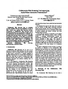
Figure 1: Overview of our interactive system. The hemispherical VEM is captured using a HDR camera with a fisheye lens. Then our importance sampling technique is used to determine a representative set of directional light sources for each VEM frame, marked by green circles in the middle image. After temporal processing the light sources are submitted to a GPU-based renderer featuring the shadow computation. the illumination of surfaces with Lambertian [Gre86], Phong [HS99], or even more general light reflectance functions [KM00]. Those techniques could be adapted for the VEM processing and they can easily support dynamic environments but ignore the visibility computation. Real-time VEM-based lighting of static scenes including shadows can be immediately performed using the precomputed radiance transfer techniques [SKS02, NRH04, LSSS04]. The limitations of static geometry (or prior animation knowledge) have been lifted for precomputed radiance transfer techniques by Kautz et al. [KLA04]. Although their method can handle only very simple scenes. HDR video texture can be used to cast realistic soft shadows for fully dynamic scenes [AAM03]. However, time consuming and memory intensive preprocessing of each video frame is required to achieve real-time rendering performance. The most common interactive rendering techniques are developed for graphics hardware, which can natively support shadows cast by point or directional light sources only. From a performance point of view it is thus desirable that captured environment maps are decomposed into a set of representative directional light sources. Several techniques based on the concept of importance sampling have been recently proposed to perform such a decomposition for static lighting [ARBJ03,KK03,ODJ04]. Unfortunately, their direct extension for VEM is usually not feasible due to at least one of the following major problems: • Too high computational costs precluding VEM capturing and scene lighting at interactive speeds [ARBJ03, KK03]. • Lack of temporal coherence in the positioning of selected point light sources for even moderate and often local lighting changes in VEM [ARBJ03, ODJ04]. • Lack of flexibility in adapting the number of light sources to the rendered frame complexity as might be required to maintain a constant framerate [ODJ04]. The latter two problems, if not handled properly, might lead to annoying popping artifacts between frames. c The Eurographics Association 2005.
Algorithm Outline In this work we present a complete pipeline from the HDR VEM acquisition to rendering at interactive speeds (refer to Figure 1). Our major concern is the efficient processing of the acquired HDR video, which leads to a good quality rendering of dynamic environments. We propose an efficient importance sampling algorithm which leads to temporally coherent sets of light sources of progressively adjustable density. The distribution of directional light sources over the hemisphere results in a good representation of environment map lighting and the fidelity of this representation smoothly increases with the number of light sources. In order to achieve interactive framerates, we introduce novel methods that significantly accelerate shading and visibility computations for any illumination described by a large set of directional lights. We implement an algorithm on a modern graphics hardware to improve the performance of per-pixel lighting using the Phong illumination model and reduce the number of shadow map visibility tests. Paper Structure In the following section we discuss previous work on importance sampling for image-based lighting. In Section 3 we present our VEM sampling technique and we focus on the issues of sampling pattern properties and temporal coherence. Since our VEM sampling approach results in many directional light sources, in Section 4 we discuss the efficiency issues for the direct lighting computation with shadows on the graphics hardware. In Section 5 we briefly describe the implementation of our interactive pipeline from the VEM acquisition to scene lighting computations. In Section 6 we show the results obtained using our system and in Section 7 we discuss its possible applications. Finally, we conclude this work and propose some directions of future research. 2. Previous Work In this section we discuss existing illumination sampling algorithms from the standpoint of their suitability for the pro-
V. Havran, M. Smyk, G. Krawczyk, K. Myszkowski, and H.-P. Seidel / Interactive System for Dynamic Scene Lighting using Capt. Video Env. Maps
cessing of VEM at interactive speeds. In particular, we focus on the issues of temporal coherence and control over the number of samples. Accompanying video provides two case studies illustrating those issues and supporting our evaluation of recent importance sampling techniques. Gibson and Murta [GM00] have developed an optimization procedure for the selection of directional EM samples which minimize the error in the reconstruction of a shadow cast by a sphere on a plane. The method requires a reference solution, which is computed using costly Monte Carlo integration over the EM for a huge number of sample points on the plane. Also, temporal coherence is poor because the optimization procedure relies on the random selection of initial samples and is prone to getting stuck in the local minima. On the other hand, forcing temporal coherence in the initial sample selection may lead to overlooking important changes in the EM intensity. Agarwal et al. [ARBJ03] propose an algorithm for the selection of directional EM samples, which combines elements of importance and stratified sampling. Through EM thresholding and connecting regions with similar intensity, a number of samples is assigned to each such region based on its summed intensity and angular extent (importance). Small regions with high total intensity are penalized to avoid too great concentration of samples in a similar direction. The stratification is performed within each coherent region by spreading samples so that the distance of newly inserted samples is maximized in respect to all existing samples whose positions remain unchanged. This enables easy control over the sample number and smooth integration with renderers performing progressive refinement of the image quality. For VEMs the algorithm leads to temporally incoherent changes in the illumination sample directions. Even local changes in some EM regions may lead to different thresholding which may affect the whole map. The computation speed is of the order of tens of seconds for a single EM. Kollig and Keller [KK03] based their algorithm on Lloyd’s relaxation method. At each iteration they insert a new sample direction near the direction representing an EM region with the highest total intensity. This may lead to a high concentration of samples around the EM regions with high intensity and small angular extents, which may reduce the performance of shadow computation during rendering. On the other hand, the differences between sample intensities are small, which reduces the variance in the lighting computation. The resulting sample distribution over the EM is smoothly changing, which leads to images of very good and stable quality even when the number of samples is moderate. The total number of samples is easy to control but adding new samples affects the positions of virtually all previously inserted samples. In the animation context even local changes in some EM regions involve global changes of sam-
ple positions in the whole map. The computation speed is of the order of tens of seconds for a single EM. Ostromoukhov et al. [ODJ04] have proposed a hierarchical importance sampling algorithm, which is based on the Penrose tiling. A hierarchical domain subdivision and its aperiodicity are inherent features of the Penrose tiling. For localized changes in the EM, the algorithm leads to very local changes of tiling. This makes this algorithm attractive for animations because temporal coherence between samples is quite good. For fully dynamic EM (e.g., captured for freely moving HDR camera) the tiling structure remains rigid and the position of light sources do not change, which results in switching the light sources on and off depending on local intensity at a given moment of time. The most serious problem with this algorithm is difficult control of the number of samples, which may change from frame to frame and significantly depends on changes in the VEM. The computation speed of the order of milliseconds for a single EM is very attractive for real-time applications. In Figure 6 we show the images from progressive rendering using above discussed methods and here presented technique. The light sources were computed off-line for [ARBJ03] and [KK03]. The images for increasing number of light sources indicate that our method is more suitable for progressive rendering thanks to the severe reduction of flickering while adding light sources than previously published methods.
3. Inverse Transform Method If the pixel intensities in the EM can be seen as a discrete 2D probability density function (PDF), the sample selection can be performed using the machinery developed in statistics. The problem of drawing samples from an arbitrary distribution is well elaborated in Monte Carlo literature [Fis96] and various practical methods such as rejection sampling or inverse transform methods have been used in computer graphics as well [DBB03]. The images as PDFs have been considered in non-photo realistic rendering applications for distributing stipples according to image intensities [SHS02]. More general approaches such as multiple-importance sampling [VG95], bidirectional importance sampling [Bur04], or various combinations of correlated and importance sampling [SSSK04] can be considered. Those approaches enable to consider also the reflectance characteristics of illuminated objects and visibility relations to choose an optimal set of illumination directions for each sample point (or the normal vector direction). However, those approaches are not currently suitable for interactive applications on graphics hardware due to their high algorithmic and computational complexity. c The Eurographics Association 2005.
V. Havran, M. Smyk, G. Krawczyk, K. Myszkowski, and H.-P. Seidel / Interactive System for Dynamic Scene Lighting using Capt. Video Env. Maps
3.1. Method Description Recently, the standard inversion procedure [Fis96] for a piecewise constant image function has been successfully applied for efficient importance sampling of a static EM [PH04, Bur04]. At first the EM is mapped into a 2D intensity image and the corresponding PDF is created. The intensity of pixels is multiplied by sin(θ), where θ denotes the altitude angle in the EM, to account for smaller angular extent of pixels around the poles. For each scanline corresponding to a discrete value of θ the cumulative distribution function (CDF) is built, which is used for the selection of the azimuth angle φ (so the brightest pixels in the scanline are more likely to be selected). Then the marginal PDF is computed based on the average intensity of each scanline and it is integrated into the CDF, which is then used for the θ angle selection (so the scanlines with the highest average intensity are more likely to be selected). Finally, samples drawn with a uniform probability distribution over the unit square are transformed via the corresponding CDFs first into the sampling direction θ (selecting a scanline) and then into the sampling direction φ (selecting a pixel within the scanline). In this work we also use PDF-based importance sampling of the EM. However, we select the inverse transform method proposed by Havran et al. [HDS03], which exhibits better continuity and uniformity properties than the standard inversion procedure used by [PH04, Bur04]. First of all it guarantees the bijectivity and continuity property for any nonnegative PDF over a hemisphere, which means that a small change in the input sample position over the unit square is always transformed into a small change in the resulting position of light source over the EM hemisphere (for the inverse transformation this property holds as well). This property is important for the relaxation of input sample positions to achieve sampling properties closer to blue noise (refer to Section 3.2). The better uniformity property leads to a better stratification of the resulting light source directions. For the details of the inverse transform approach developed by Havran et al. we refer the reader to [HDS03], we recall the method here only briefly. The mapping consists of four stages. At first, samples are mapped from a unit square into a unit disc parametrized with radius rd and angle φd using the method of concentric maps [SC97]. The second and third stages correspond to drawing a sample from the disc using 1D CDFs which are defined over the rd and φd parameter space. The continuity of those mappings is preserved using a linear interpolation between neighboring 1D CDFs. Finally, the samples from the disc are mapped to the hemisphere so that the differential surface areas are preserved. For VEM applications both the standard and Havran’s inverse transform methods are perfectly suitable in terms of the computation performance. The standard method is slightly faster, but for drawing a moderate number of samples (less than 1,000 in our application) the computation time differences are negligible. The main costs for both c The Eurographics Association 2005.
(a)
(b)
(c)
Figure 2: Transform of the tiled unit square (a) using the standard (top row) and Havran’s (bottom row) inverse transform methods for various PDF functions: (b) uniform and (c) a sky probe.
methods are incurred by the CDF computation. Figure 2 shows the results of transformation of a tiled unit square using the standard and Havran’s inverse transform algorithms for various types of EM. As can be seen Havran’s method leads to a better regularity and compactness of the transformed tiles, which results in better stratification properties in lighting sample distribution. The key feature of Havran’s method is the first step of concentric mapping [SC97], which reduces distortions and removes continuity problems. In contrast, the standard method may exhibit some problems with the sample motion continuity, which is especially problematic for trajectories traversing the border for φ = 0 (marked in Figure 2 as the red line spanning between the hemisphere pole and the horizon). Also, samples tend to move more along the hemisphere parallels and stay away from the hemisphere pole. An important issue in extending the inverse transform method to handle dynamic image sequences is to improve temporal coherence in importance sampling. The most obvious step towards this goal is to choose the same set of initial samples over the unit square for each VEM frame. There are various possible choices of sampling patterns, which may lead to a different quality of the reconstructed lighting. In Section 3.2 we describe our approach which features a good sample stratification over the EM while retaining progressive control over the number of samples. Since even local changes in the EM lead to global changes of the PDF, the direction of virtually all light sources may change from frame to frame which causes unpleasant flickering in the rendered images. In Section 3.3 we discuss our solutions towards reducing this problem through improving temporal coherence in the importance sampling.
V. Havran, M. Smyk, G. Krawczyk, K. Myszkowski, and H.-P. Seidel / Interactive System for Dynamic Scene Lighting using Capt. Video Env. Maps
3.2. Sampling Pattern Properties The problem of sampling pattern selection over a unit square is well studied [Nie92, Gla95]. Since our emphasis is on interactive applications we would like to use a progressive sequence of sample points in which adding new points does not affect the position of points used for the previous VEM frame, while good sampling properties are retained. Obviously, this assumption holds when points are removed as well. All algorithms involving re-arranging sample points after each such a change are not acceptable due to excessive image flickering. We achieve the progressiveness goal using quasi-Monte Carlo sequences such as the Halton sequence or in general (0, s)-sequences [Nie92]. Those sequences naturally lead to a good stratification of the sampling domain for successively added samples from the sequence. We use the 2D Halton sequence with bases p1 = 2 and p2 = 3, whose discrepancy is the lowest for the number of samples N = p1 k1 · p2 k2 , where k1 and k2 are nonnegative integers. This means that considering other sample numbers than N leads to worse sampling properties, but a good stratification is still obtained even when subsequent samples are added. We can easily correct the position of the Halton points on the 2D square to achieve the blue noise sampling pattern as recommended by Ostromoukhov et al. [ODJ04] to reduce aliasing artifacts. For this purpose Lloyd’s relaxation over the initial sample positions can be performed [HDK01] at the preprocessing stage and then the resulting samples can be used for all VEM. Blue noise properties of the sampling pattern over the hemisphere can be affected as a result of the inverse transform method, especially in regions in which the PDF changes abruptly. The continuity of mapping from the 2D square to the 3D hemisphere obtained using Havran’s algorithm is crucial towards preserving a good approximation of blue noise sampling in the regions of low PDF variation. Figure 3 shows the sample point stratification with/without blue noise properties over the hemisphere as a results of the standard and Havran inverse transforms for the uniform PDF. In our application, where we use the samples for integration, the blue noise of a sampling pattern results in a slightly better isotropic uniformity than a pure Halton sequence. The achieved progressiveness of the sampling pattern can be used in two ways. The number of samples can be adaptively adjusted to keep the framerate constant, while keeping the variance resulting form such changes low due to good stratification properties. Also, in progressive rendering the image quality can be smoothly improved by increasing the number of considered lights (this requires freezing the VEM frame). 3.3. Handling Dynamic Sequences The dynamic VEM lighting represented by a limited number of directional light sources moving over the hemisphere
Figure 3: Sampling pattern resulting from applying the standard (left column) and Havran (right column) inverse transform methods to the original (upper row) and relaxed to blue noise (bottom row) 2D Halton sequences. A uniform PDF is assumed for this transformation. The sample point distribution is shown using the hemispherical mapping.
is prone to flickering artifacts in rendering. Therefore, improving temporal coherence for each directional light is very important, which we want to achieve through filtering of a signal related to the light sources. The question arises how the signal is in fact represented and how it should be filtered in our application. In the traditional view to an 1D discrete signal in signal processing [OSB99], a signal is represented by changes of the amplitude in time. In our context the signal corresponding to directional light sources is represented by both changes of the power and the position of the light sources from frame to frame. This creates two sources of flickering that should be dealt with independently. The first source of real-world VEM capturing flickering is caused by changes of the light source power from frame to frame, e.g., when the VEM capturing is performed in an interior with fluorescent lighting. In this case the total lighting power is our temporal signal and the temporal filter application is straightforward. We compute the power emanated from EM for every frame and this is used as the input of filtering. As a result of filtering the overall energy in the system is preserved, which is naturally achieved through normalizing the filter weighting coefficients. It follows from the importance sampling described above that all the light sources have the same power in a single frame. The second source of flickering is due to abrupt and often jumpy changes in the position of directional light sources from frame to frame. This affects the reflected light intensity and shadow positions. Because of this dependency, the light position is our signal in temporal domain and we apply our c The Eurographics Association 2005.
V. Havran, M. Smyk, G. Krawczyk, K. Myszkowski, and H.-P. Seidel / Interactive System for Dynamic Scene Lighting using Capt. Video Env. Maps
filtering to the trajectory of each light motion over the hemisphere. The direction of a light source is filtered in 3D vector space followed by normalization to a unit vector.
cations [Win05]. Since frame grabbing in our system works asynchronously in respect to usually slower rendering, the delay is even less noticeable in our application.
The relation between a light source position and reflected lighting intensity depends directly on the incoming light direction and surface reflectance function. Thus eliminating high frequencies from the light source motion trajectory leads also to an elimination of such frequencies in the reflected lighting. In the case of shadows, the problem is more complicated because the velocity of a moving shadow must be estimated, which depends on the spatial positioning of the light occluder and receiver. It can be shown [Wat86, Win05] that a 2D shadow pattern characterized by the spatial frequencies ρ1 and ρ2 and moving along the image plane with the velocity ~v is equivalent to the visual pattern of the same spatial frequencies and blinking with temporal frequency ω:
Note that our filtering approach requires tracking of the same directional light for subsequent frames which is easy for our samples with unique positions in the unit square and indexed by the Halton sequence (refer to Section 3.2). Assigning such indices to directional lights would be difficult for the importance sampling methods discussed in Section 2.
ω = vx ρ1 + vy ρ2 =~v ·~ρ
(1)
While this relationship between flickering and the shadow motion is more complex, the shadow velocity still depends on changes in the light source position which is processed by filtering in temporal domain. In our choice for filtering mechanism we exploit limitations of the human visual system in terms of the temporal frequency response, which can be characterized by two modes: transient (bandpass for stimuli with low spatial frequency) and sustained (lowpass for stimuli with high spatial frequency) [Wat86]. To model the full human visual system behavior usually two separate filters for each of those modes are applied on a signal in the time domain. Since our lighting flickering artifacts contain mainly high temporal frequencies, we use only the lowpass filter. While our filter design is inspired by perceptual considerations, we apply a far more aggressive cut-off of the high frequencies at the level of 10 Hz to attenuate the signal, which would otherwise be improperly reconstructed causing temporal aliasing (the rate of VEM frame grabbing is about 21 Hz).
4. Improving Rendering Performance Efficient illumination computation for a large number of directional light sources arising from the EM importance sampling is a difficult problem which has been mostly addressed for static lighting. Various forms of coherence in spatial and angular domains have been explored and lead to a significant reduction in the visibility computation for off-line rendering. We are aiming at an interactive algorithm which can work for VEM and is suitable for graphics hardware implementation. In the following section we propose an approach for fast selection of those light sources which contribute to the illumination of a given point. We then extend this general algorithm to handle specifically glossy surfaces. We also present a light source clustering algorithm to reduce the shadow computation cost during rendering. 4.1. Eliminating Invisible Lights
For filtering of a signal we can use finite impulse response (FIR) or infinite impulse response (IIR) filters, which are standard tools in digital signal processing [OSB99]. We choose the FIR equiripple filter [OSB99] of order 8 (9 coefficients) designed using the filter design tool in Matlab Signal Processing Toolbox [Mat04] for the sampling frequency 21 Hz, the pass frequency 7 Hz and the stop frequency 9 Hz. The weighting coefficients of the filter are: w1 = w9 = 0.06216, w2 = w8 = 0.01296, w3 = w7 = −0.13816, w4 = w6 = 0.28315, and w5 = 0.65223. The used FIR filter leads to a delay of 4 VEM frames. We used this filter in all the cases, although we tested also several other FIR filters. The different capturing framerate and different rendering framerate could require redesigning the filter.
Under the distant lighting assumption a subset of directional light sources contributing to the illumination of all points in the scene, which feature the same normal vector direction can be uniquely determined. This observation can be easily extended for an arbitrary angular range of normal vector directions. We use those observations for a fast identification of contributing light sources. We cover the spherical surface by overlapping angular regions using a set of precomputed normals, which are uniformly distributed on the sphere (refer to Figure 4 (a)). Every angular region is defined by its center ~P and the size of the angular region measured in the maximum angular distance β. If the maximum angular distance between the centers of any neighboring angular regions is α/2, then the maximum angular distance covered by the angular region is given as β = α/2 + π/2. For a surface normal ~N of a shaded point we locate a corresponding angular region, for which we precompute the set of light sources. This efficiently culls off the majority of the invisible light sources. Theoretically, the maximum speedup that can be achieved using this technique is on average 2 for the sphere (β = π/2). Since we use a moderate number of angular regions, a practical speedup usually falls into the range of 1.6–1.8.
Even shorter delay could be achieved using IIR filters. However, we decided to use FIR filters which feature linear phase that is often desirable for video processing appli-
In the preprocessing, the light sources are distributed to all angular regions which cover the light source directions. Every light source is assigned to several overlapping angular
c The Eurographics Association 2005.
V. Havran, M. Smyk, G. Krawczyk, K. Myszkowski, and H.-P. Seidel / Interactive System for Dynamic Scene Lighting using Capt. Video Env. Maps
regions. During rendering, we use a lookup table (LUT) addressed by the normal at a shaded point to find in a constant time the corresponding angular region. We compute the illumination only for the light sources assigned to the angular region. Some light sources are still eliminated online since β > π/2. An important property of our construction is the propagation of our sampling progressiveness (refer to Section 3.2) to the angular regions: Observation 1: The samples drawn progressively according to the importance function F in the domain D are also drawn progressively in any continuous subdomain of the domain D. Note that the progressiveness of sampling pattern is inherent to (0, 1)-sequences and thus also to the Halton sequence. An intuitive justification for the above observation is as follows. Let the integrand of importance sampling function F over the whole domain be Iw and over a subdomain Is . If the sampling scheme is progressive and follows F, the number of samples in the subdomain can be estimated as Ks ≈ K · Is /Iw , where K is the total number of samples (with limK→∞ Ks /K = Is /Iw ). Since the ordering of samples in the subdomain is preserved, the samples in the subdomain are also drawn progressively. The set of directions for angular regions and the LUT are fixed before rendering. The angular region is found for both preprocessing and rendering using a LUT discretizing the sphere on faces of a cube. This can be efficiently implemented both on CPU and GPU. The proposed technique can also be used for off-line rendering involving many directional light sources based on ray tracing etc. 4.2. Handling Glossy Surfaces We use Observation 1 to improve the quality for rendering of glossy surfaces as well. In the lighting computation we consider those directional light sources which overlap with the direction of a specular lobe of BRDF determined for the surface normal and a given view direction. We precompute two sets of light sources: L and H of low and high intensities IL and IH , respectively (|L| � |H| and IL � IH ). To generate the direction of these light sources in both sets we use the relaxed samples of Halton sequence of length |L| (refer to Section 3.2) as the input of inverse transform method. For light sources in H we use a subsequence from L with the re-scaled light source power. We use two different sets SL and SH of angular regions (similar as those described in Section 4.1) for light sets L and H, respectively. In general for angular regions in SH we can use a different set of the normals to trade-off the rendering quality and preprocessing time. The set SH corresponds to eliminating the invisible light sources as described above. The set SL of angular regions is used to improve the estimate in the direction of the specular lobe. We assume that
the minimum angular distance between the centers of two (neighboring) angular regions in SL is γ. We set the size of the angular region also to γ, so the angular regions in SL are overlapping. This is depicted in Figure 4 (b). Prior to shading computation we determine the ideally reflected direction ~R for the viewing direction ~V and the normal ~N. Then the computation is carried out in two stages. First, we sum up the contributions from SL which belong to the cone C given by ~R and angular distance γ/2. Second, we add the contributions from SH that do not belong to the cone C (refer to Figure 4 (c)). The technique can be seen as a simple variant of stratified importance sampling with two strata that are handled independently. The first strata corresponds to the box window (cone C) for the sample set L. The second strata is the complement of the box window for the sample set H. In this way we improve the estimate locally inside the cone C that is important for glossy surfaces. Since we generate H as a subsequence L, the positions of SH are contained in SL . Hence we minimize possible artifacts on the boundaries in shading for an assignment to two neighboring pixels belonging to two neighboring cones. If the number of light sources in a cone C is too high and it could decrease the rendering speed significantly, we pick up only the first k light sources belonging to C and scale up their power appropriately. Above introduced Observation 1 is applied here as well to keep the progressiveness of our sampling pattern inside the cone. 4.3. Lights Clustering Another way to improve the rendering speed is the clustering of light sources with similar directions. Since we work with the directional light sources, we do not need any spatial hierarchy [PPD98]. We impose two major requirements on the light source clustering: Real-time performance and whenever possible maintaining the progressiveness. The clustering can significantly decrease the computation time for scenes with a few strong light sources. As the input for clustering an ordered sequence of light sources with the same base intensity is provided. As the output the ordered sequence of clustered light sources with a larger (or equal) intensity than the base one is obtained. Our clustering algorithm is based on the bounding box decomposition tree of Arya et al. [AMN∗ 94] that offers an optimal performance for approximate searches over arbitrarily distributed point data. Let us assume that the maximum number of light sources after clustering on the hemisphere is Q. If the light sources after clustering would cover uniformly the hemisphere, then each cluster has to cover the solid angle 2 · π/Q. In terms of the size of angular region ε each cluster covers the solid angle π · sin2 (ε). From p that we can compute that the angular distance ε = c f · arcsin 2/Q. The coefficient c f is the correction factor to account for covering of hemisphere by the circular discs (c f ≈ 1.8 − 1.9). c The Eurographics Association 2005.
V. Havran, M. Smyk, G. Krawczyk, K. Myszkowski, and H.-P. Seidel / Interactive System for Dynamic Scene Lighting using Capt. Video Env. Maps
(a)
(b)
(c)
Figure 4: Selection of relevant light sources for the shadow computation (a) Eliminating invisible lights: Only the lights in the angular region marked in yellow are used for shading of a point, whose normal lies in the cone with the center ~P and the angular extent α/2. (b) Handling glossy surfaces: The high intensity light sources in the set H are refined to low intensity light sources creating the set L. The light sources from L are distributed into narrower overlapping angular regions A 1 , A2 , and A3 marked in red, blue, and green. (c) A situation for a reflected ray ~R: The low intensity light sources from the angular region A2 inside the cone C are used. Also, the high intensity light sources outside the cone C are used. The cone A 2 is found using a LUT addressed by the reflected ray ~R.
The clustering processes all the light sources one by one starting with the first light source in the input sequence. We search all the light sources within the angular distance ε and add them to the cluster. The minimum number of light sources in every cluster is one. After assigning all the light sources to the clusters we compute representative light source directions for each cluster by averaging the direction all the light sources assigned to the cluster. The proposed way of the construction improves the temporal stability of resulting light source sequence in time, since the selection of the cluster centers is more temporally coherent than a random algorithm. The clustering is hardly compliant with progressiveness and it increases variance of the estimated illumination, since the light sources have unequal power after the clustering. For graphics hardware with framerate constraints it pays off to use clustering for the VEM, since the number of light sources after clustering is bounded by the user selected Q. The price to be paid for the performance improvements by clustering is decreased quality of shadows and specular reflections. We use the clustering only for high intensity light sources in set H.
5. Implementation The design of the whole system for capturing, light source computation, and rendering was driven by the following aspects: c The Eurographics Association 2005.
• Computations should be optimally distributed between CPU and GPU on a single PC. • System should respond interactively. • Visualization technique may not involve any precomputations and therefore should allow to render an arbitrary geometry. The system pipeline is illustrated in Figure 5. The input to the system are the VEM from the HDR video camera and scene geometry. The light source generation is performed on CPU in synchronization with the camera, while the rendering is performed asynchronously almost completely on GPU. Since the rendering on GPU is slower than processing of environment maps on CPU, the delay introduced by the temporal FIR filter is effectively reduced. 5.1. HDR Acquisition According to the specification of the HDRC VGAx (IMS CHIPS) sensor, the video camera used in our experiments has a logarithmic response. Following this assumption, we performed the photometric calibration by acquiring six gray patches of known luminance, and fitting the measured data versus the camera output values to a logarithmic function. Two other measurements were used to assess the quality of the fit and proved that the calibration was sufficiently correct. Such photometric calibration is required to faithfully represent the illumination of the captured environment. It is also worth to note that the camera is able to capture eight orders of light intensity magnitude (at constant aperture and no gain control) leading to saturation-free images.
V. Havran, M. Smyk, G. Krawczyk, K. Myszkowski, and H.-P. Seidel / Interactive System for Dynamic Scene Lighting using Capt. Video Env. Maps
The implementation divides the sphere uniformly into angular regions Ai . A cube-map texture that maps these regions to integer values is constructed, so that one lookup is enough to transform a vector into a number of the region it belongs to. During frame preprocessing we associate every region Ai with a set of light sources H than can potentially influence the surfaces with the normal vector contained within Ai . For a Lambertian surface the set of potential contributors includes all light sources located on the hemisphere above it and also those a few degrees below the horizon (where the exact angle depends on the area of Ai ), but for BRDFs with large specular peaks it makes sense to only allow lights that are located within a narrow cone around the central direction of Ai . This information is encoded on the fly in a texture TexL, one region per row. Each light source is represented by RGB values, and by its XY Z direction. If shadows are enabled, the alpha channel value stores the shadow ID (refer to Section 5.2.1).
Figure 5: The system pipeline illustrating the distribution of tasks between CPU and GPU.
In addition, the environment map captured using a fisheye lens has to be transformed to the uniform polar coordinates for the importance sampling. The necessary geometric calibration is performed according to a generic fisheye lens model [KB04]. To enable proper visualization of HDR data, we implemented the global version of [RSSF02] tone mapping algorithm. In order to prevent the temporal aliasing artifacts visible as brightness flickering, we extended the algorithm to temporal domain by smoothing its two parameters over time: the world luminance and the key value. The tone mapping is implemented as a fragment program and is performed as a separate rendering pass. 5.2. Rendering System Our rendering subsystem is built using OpenGL and Cg, and supports per-pixel lighting, non-diffuse BRDFs, a few thousands directional light sources, and up to hundreds of independent shadows. The rendering is performed in two stages: shadow map preparation and geometry visualization, which is carried out in a single pass. In order to properly support highly varying lighting conditions that require a large number of directional light sources we make use of light elimination technique described in Section 4.1. This allows us to support few thousands of light sources, greatly facilitating illumination computation on highly glossy surfaces.
Performance-wise, a naive algorithm manages to distribute several hundreds of lights below one millisecond, processing larger numbers may be realized with a LUT indexed by the normal vector. The illumination computations take place in a pixel shader, which uses normal (for diffuse) or reflected (for specular) vector to perform a cube-map lookup locating a row in TexL that contains information about lights relevant for the current pixel. It then walks along the row and accumulates contributions from all light sources present in it, including BRDF processing. This procedure is performed twice: first, for diffuse illumination with light sources in set H and then for specular illumination with light sources in set L, while special care is taken to avoid summing energy twice (refer to Section 4.2). 5.2.1. Shadows When reconstructing a diffuse part of the illumination we have the option of using shadows, realized using shadow maps. For a glossy/specular part we select the most relevant shadow map from the above set. Since generating hundreds of shadow maps can put a heavy burden even on a modern graphics hardware, we make several steps in order to improve the rendering performance. To avoid expensive render target switches, as well as to conserve texturing units of the GPU, we render all shadow maps to one large texture. The texture is of square size, with shadow maps organized into a grid. Each shadow map requires separate 4 × 4 matrix which transforms it into the current view in order to make depth comparisons possible. There is not enough constant registers to pass all these matrices to fragment program and encoding them in the texture would result in 4 × 72 float RGBA texc The Eurographics Association 2005.
V. Havran, M. Smyk, G. Krawczyk, K. Myszkowski, and H.-P. Seidel / Interactive System for Dynamic Scene Lighting using Capt. Video Env. Maps
ture reads (or half of it using packed representation), thus severely impacting the performance. Instead, we only pass light projection matrix (which is shared by all shadow maps) as a parameter and reconstruct the remaining transformation matrices on the fly in the fragment program, basically implementing functionality of glutLookAt(). The only variable in such case is the direction to the light, which means 72 float RGBA texture accesses. However, these do not incur any additional cost, as light directions are accessed anyway in the illumination pass (Section 5.2). To exploit this, information about a light stored in TexL can also contain an index of this light’s shadow map within the shadow texture. If this index is present, the shadow map transformation matrix is constructed and the range check is performed. It is thus possible to address a large number of shadow maps using one texturing unit in a single rendering pass.
6. Results Below we provide the performance results of the proposed system obtained on the following hardware: a PC with 3 GHz Pentium4 with 512kB L2 cache equipped with NVidia GeForce 6800GT. Currently, the system is limited by the frame grabber and camera capture rate and by the performance of graphics hardware. The rendering time on GPU is proportional to the resolution of the image and the number of the directional light sources used. The computation time of CPU and GPU is spent on the following tasks. Capturing the image data from the frame grabber and converting it to the polar projection of the resolution 360×90 pixels takes below 1 ms. The precomputation of the CDF and the luminous power emitted by the current frame of VEM is below 2 ms. The samples are computed at the rate of 410 samples/ms. Temporal filtering with the FIR order 8 filter requires 1 ms for 210 directional light sources. Optional clustering requires about 1 ms to process 300 light sources. The precomputation of the textures for 200 angular regions takes below 1 ms. The total time for computing 300 directional light sources with temporal processing and clustering is below 5 ms. The computation bottleneck on the GPU is in the pixel shader and the rendering time also depends on the properties of objects’ BRDF. For this reason we have used only 72 light sources in set H and maximally 216 light sources for every angular region in set SL . Also the shadow maps number was limited to 72. The resolution of a single shadow map was set 256×256, allowing to organize 72 shadow maps in a texture 2,304×2,304 pixels in a 9×9 grid (the last row is unused). Below we give the results for rendering performance at the image resolution 320×240 pixel. For rendering without the angular regions described in Section 4.1 we achieve framerate from 7 Hz for Lambertian surface decreased to 3.9 Hz, c The Eurographics Association 2005.
when a special handling for glossy surfaces is used (Section 4.2). The rendering speed is increased by 70% when angular regions are used to cull off the invisible light sources. The examples of the rendered images grabbed in real time are shown in Figures 7 and 8. As expected the clustering of light sources described in Section 4.3 increases the rendering speed significantly in the detriment of the image quality. We observed speedups by up to 200% for a common office lighting and outdoor illumination with strong sunlight. 7. Discussion Our system has many potential applications in mixed reality applications and virtual studio systems. So far dynamic lighting in such systems is performed by scripting rigidly set matrices of light sources whose changes are synchronized with the virtual set rendering. Such systems are expensive and require significant human assistance, which reduces their applicability for smaller broadcasters. Our approach can support arbitrary changes of lighting in virtual studio in a fully automatic way. One important application area with a large growth potential is augmented reality, where synthetic entities are expected to blend seamlessly with the real world surroundings, objects and persons. Mobile systems built on principles similar to ours could for instance be used in outdoor television, enabling virtual characters to leave confines of studio environment. The decomposition of intensity represented by a VEM into a set of directional light sources can also be considered as a method of compressing lighting information suitable for the low-bandwidth transmission, which enables relighting in a remote location. The level of compression can be smoothly controlled by changing the number of lights due to their good stratification and ordering properties (refer to Section 3.2). 8. Conclusions We presented a system for interactive capturing of high dynamic range video environment maps, which are used for immediate lighting of dynamic scenes. We proposed an efficient algorithm for importance sampling of the lighting intensity function in subsequent video frames, which features a good temporal coherence and spatial distribution properties (stratification) of resulting directional light sources. To keep a constant framerate or enable progressive image quality enhancement, the number of those lights can be easily controlled on the fly while good sample stratification properties are always preserved. The integrated OpenGL based renderer using our new technique for discarding irrelevant lights and exploiting features of modern graphics hardware like programmable, per-pixel shading was able to deliver interactive framerates using a single PC-class machine and a consumer level video card.
V. Havran, M. Smyk, G. Krawczyk, K. Myszkowski, and H.-P. Seidel / Interactive System for Dynamic Scene Lighting using Capt. Video Env. Maps
Figure 6: Comparison of the image quality as the result of adding light sources for the methods proposed by Agarwal et al., Kollig and Keller, Ostromoukhov et al., and us. We consider decomposition of the EM into 4, 8, 16, 32, 64, and 128 light sources. Notice that even for a small number of light sources the quality of shadow reconstruction in respect to the solution with 128 lights, which is visually indistinguishable from reference solution, is the best for Kollig and Keller and our method.
Our system lifts common limitations of existing rendering techniques which cannot handle at interactive speeds HDR image-based lighting captured in dynamic real world conditions along with complex shadows, fully dynamic geometry, and arbitrary reflectance models. Our approach does not require any costly preprocessing and has modest memory requirements to achieve those goals. As future work we want to lift the assumption of distant lighting by adding to our system one or more spatially distributed HDR cameras with the fisheye lenses. Based on the known distance between each pair of cameras, the positions of nearly located light sources could be determined on the fly as similarly proposed by Sato et al. [SSI99], and such lights could be then represented as the point light sources during rendering instead of currently used directional lights. Also, we want to extend our system for mixed reality applications in which dynamic changes of lighting, geometry, and camera must be supported. In terms of the lighting computation, what remains to be done is to model the impact of synthetic objects on lighting in the real world environment. Acknowledgments We would like to thank Philipp Jenke for his proofreading the previous version of the paper and Kristina Scherbaum and Josef Zajac for their help with illustrations. Further, we would like to thank Paul Debevec and Andrew Jones for providing us with a sequence of HDR images of the sky which
we have used for testing our techniques. This work was partially supported by the European Union within the scope of project IST-2001-34744, “Realtime Visualization of Complex Reflectance Behaviour in Virtual Prototyping” (RealReflect). References [AAM03] A SSARSSON U., A KENINE -M ÖLLER T.: A Geometry-Based Soft Shadow Volume Algorithm using Graphics Hardware. ACM Transactions on Graphics 22, 3 (2003), 511–520. 3 [AMN∗ 94]
A RYA S., M OUNT D. M., N ETANYAHU N. S., S IL R., W U A. Y.: An Optimal Algorithm for Approximate Nearest Neighbor Searching. In SODA (1994), pp. 573– 582. 8 VERMAN
[ARBJ03] AGARWAL S., R AMAMOORTHI R., B ELONGIE S., J ENSEN H. W.: Structured Importance Sampling of Environment Maps. ACM Transactions on Graphics 22, 3 (2003), 605–612. 3, 4 [Bur04] B URKE P. S.: Bidirectional Importance Sampling for Illumination from Environment Maps. M.sc. thesis, Computer Science Department, University of British Columbia (October, 22), 2004. 4, 5 [DBB03] D UTRÉ P., B EKAERT P., BALA K.: Advanced Global illumination. A K Peters, Natick, Massachusetts, 2003. 4 [Deb98] D EBEVEC P.: Rendering Synthetic Objects Into Real Scenes: Bridging Traditional and Image-Based Graphics With c The Eurographics Association 2005.
V. Havran, M. Smyk, G. Krawczyk, K. Myszkowski, and H.-P. Seidel / Interactive System for Dynamic Scene Lighting using Capt. Video Env. Maps Global Illumination and High Dynamic Range Photography. In Proceedings of SIGGRAPH 98 (1998), Computer Graphics Proceedings, Annual Conference Series, pp. 189–198. 2
[Nie92] N IEDERREITER H.: Random Number Generation and Quasi-Monte Carlo Methods. Society for Industrial and Applied Mathematics, 1992. 6
[DM97] D EBEVEC P. E., M ALIK J.: Recovering High Dynamic Range Radiance Maps from Photographs. In Proceedings of SIGGRAPH 97 (1997), Computer Graphics Proceedings, Annual Conference Series, pp. 369–378. 2
[NRH04] N G R., R AMAMOORTHI R., H ANRAHAN P.: Triple Product Wavelet Integrals for All-Frequency Relighting. ACM Transactions on Graphics 23, 3 (2004), 477–487. 3
[FDA03] F LEMING R., D ROR R., A DELSON E.: Real-World Illumination and the Perception of Surface Reflectance Properties. Journal of Vision 3, 5 (2003), 347–368. 2 [Fis96] F ISHMAN G. S.: Monte Carlo: Concepts, Algorithms, and Applications. Springer-Verlag, New York, NY, 1996. 4, 5 [Gla95] G LASSNER A. S.: Principles of Digital Image Synthesis. Morgan Kaufmann, San Francisco, CA, 1995. 6 [GM00] G IBSON S., M URTA A.: Interactive Rendering with Real World Illumination. In Rendering Techniques 2000: 11th Eurographics Workshop on Rendering (2000), pp. 365–376. 4 [Gre86] G REENE N.: Environment Mapping and Other Applications of World Projections. IEEE Computer Graphics & Applications 6, 11 (1986), 21–29. 3 [HDK01] H ILLER S., D EUSSEN O., K ELLER A.: Tiled Blue Noise Samples. In Vision, Modeling, and Visualization (2001), pp. 265–272. 6 [HDS03] H AVRAN V., D MITRIEV K., S EIDEL H.-P.: Goniometric Diagram Mapping for Hemisphere. Short Presentations (Eurographics 2003), 2003. 5 [HS99] H EIDRICH W., S EIDEL H.-P.: Realistic, HardwareAccelerated Shading and Lighting. In Proceedings of SIGGRAPH 99 (1999), Computer Graphics Proceedings, Annual Conference Series, pp. 171–178. 3 [KB04] K ANNALA J., B RANDT S.: A Generic Camera Calibration Method for Fish-Eye Lenses. In Proceedings of the 2004 Virtual Reality (2004), IEEE. 10 [KK03] KOLLIG T., K ELLER A.: Efficient Illumination by High Dynamic Range Images. In Eurographics Symposium on Rendering: 14th Eurographics Workshop on Rendering (2003), pp. 45– 51. 3, 4 [KLA04] K AUTZ J., L EHTINEN J., A ILA T.: Hemispherical Rasterization for Self-Shadowing of Dynamic Objects. In Eurographics Symposium on Rendering: 15th Eurographics Workshop on Rendering (2004), pp. 179–184. 3
[ODJ04] O STROMOUKHOV V., D ONOHUE C., J ODOIN P.-M.: Fast Hierarchical Importance Sampling with Blue Noise Properties. ACM Transactions on Graphics 23, 3 (2004), 488–495. 3, 4, 6 [OSB99] O PPENHEIM A., S CHAFER R., B UCK J.: DiscreteTime Signal Processing, 2nd edition. Prentice-Hall, Engelwoord Cliffs, NJ, 1999. 6, 7 [PH04] P HARR M., H UMPHREYS G.: Infinite Area Light Source with Importance Sampling. In an Internet publication accompanying the book Physically Based Rendering from Theory to Implementation, http://pbrt.org/plugins.php (October, 13) (2004). 5 [PPD98] PAQUETTE E., P OULIN P., D RETTAKIS G.: A Light Hierarchy for Fast Rendering of Scenes with Many Lights. Computer Graphics Journal (Proc. Eurographics ’98) 17, 3 (September 1998), C63–C74. 8 [RSSF02] R EINHARD E., S TARK M., S HIRLEY P., F ERWERDA J.: Photographic Tone Reproduction for Digital Images. ACM Transactions on Graphics 21, 3 (2002), 267–276. 10 [SC97] S HIRLEY P., C HIU K.: A Low Distortion Map Between Disk and Square. Journal of Graphics Tools 2, 3 (1997), 45–52. 5 [SHS02] S ECORD A., H EIDRICH W., S TREIT L.: Fast Primitive Distribution for Illustration. In Rendering Techniques 2002: 13th Eurographics Workshop on Rendering (2002), pp. 215–226. 4 [SKS02] S LOAN P.-P., K AUTZ J., S NYDER J.: Precomputed Radiance Transfer for Real-Time Rendering in Dynamic, LowFrequency Lighting Environments. ACM Transactions on Graphics 21, 3 (2002), 527–536. 3 [SSI99] S ATO I., S ATO Y., I KEUCHI K.: Acquiring a Radiance Distribution to Superimpose Virtual Objects onto a Real Scene. IEEE Transactions on Visualization and Computer Graphics 5, 1 (January-March 1999), 1–12. 12 [SSSK04] S ZÉCSI L., S BERT M., S ZIRMAY-K ALOS L.: Combined Correlated and Importance Sampling in Direct Light Source Computation and Environment Mapping. Computer Graphics Forum 23, 3 (2004), 585–593. 4
[KM00] K AUTZ J., M C C OOL M. D.: Approximation of Glossy Reflection with Prefiltered Environment Maps. In Graphics Interface (2000), pp. 119–126. 3
[STJ∗ 04] S TUMPFEL J., T CHOU C., J ONES A., H AWKINS T., W ENGER A., D EBEVEC P. E.: Direct HDR Capture of the Sun and Sky. In Afrigraph (2004), pp. 145–149. 2
[KUWS03] K ANG S. B., U YTTENDAELE M., W INDER S., S ZELISKI R.: High Dynamic Range Video. ACM Transactions on Graphics 22, 3 (2003), 319–325. 2
[VG95] V EACH E., G UIBAS L. J.: Optimally Combining Sampling Techniques for Monte Carlo Rendering. In Proceedings of SIGGRAPH 95 (1995), Computer Graphics Proceedings, Annual Conference Series, pp. 419–428. 4
[LSSS04] L IU X., S LOAN P.-P., S HUM H.-Y., S NYDER J.: AllFrequency Precomputed Radiance Transfer for Glossy Objects. In Eurographics Symposium on Rendering: 15th Eurographics Workshop on Rendering (June 2004), pp. 337–344. 3 [Mat04] Matlab signal processing toolbox 6.3. http://www.mathworks.com/products/signal/, 2004. 7 c The Eurographics Association 2005.
[Wat86] WATSON A.: Temporal Sensitivity. In Handbook of Perception and Human Performance, Chapter 6 (1986), John Wiley, New York. 7 [Win05] W INKLER S.: Digital Video Quality: Vision Models and Metrics. John Wiley & Sons, Ltd, West Sussex, England, 2005. 7
V. Havran, M. Smyk, G. Krawczyk, K. Myszkowski, and H.-P. Seidel / Interactive System for Dynamic Scene Lighting using Capt. Video Env. Maps
camera
Figure 7: (top) the model covered by specular BRDF with 16,200 triangles rendered with 72 shadow maps at 5.3 Hz. On the left top is an environment map captured in real-time as captured through fisheye lens HDR camera. The light sources are marked by green points. On the left bottom the same environment map is shown in polar projection. (bottom) the same model illuminated by outdoor lighting.
Figure 8: Comparison of the fidelity in the shadow and lighting reconstruction for the real-world and synthetic angel statuette illuminated by dynamic lighting. Real-world lighting is captured by the HDR video camera located in the front of the round table with an angel statuette placed atop (the right image side). The captured lighting is used to illuminate the synthetic model of the angel statuette shown in the display (the left image side).
c The Eurographics Association 2005.