Interactive, Task-Oriented Visualizations to Explore Decay Chain Calculation Martin Eller1,2, Silvia Miksch2,3, Jacques Lettry1 European Organization for Nuclear Research (CERN) 2 Institute of Software Technology and Interactive Systems (Vienna University of Technology) 3 Danube University Krems {
[email protected],
[email protected],
[email protected]} 1
Abstract Most applications in physical calculations provide powerful multivariate outputs but use rather simple visual representations (diagrams) without the possibilities to explore the resulting data sets. Interdependences in the data are overlooked or stay unseen and the analysis is very time-consuming, because of the difficulty and complexity for users to grasp the results. In this paper we present a tool which combines a visual structure recognised by the physical community with interactive information visualization techniques to support the analysis of decay chain calculations. In a case study we showed that our tool helped experts in the field to analyse radioactive decay chains where the representation of results is more concise and conclusions are easier drawn.
(see Section 4) and the nuclide chart [13] (see Section 3). They are well known and need no explanation in the physical community. We explain how we adapted the nuclide chart and introduce additional diagrams to support cognition. Interactions are important to improve the understanding of results. In Section 4 we describe various interaction techniques to tune the visualization. For time-oriented data exploration we propose animations over time. First results and further application scenarios are presented in Section 5.
2. Values and Dimensions The data base for our case study consists of data derived from simulation or calculation programs. The programs implement either formulas, statistical methods, or are based on measurements. The resulting output has to be acquired or imported from a database or has to be converted to fit our file standard.
1. Introduction
2.1. Thousands of Isotopes and Target Materials
There are various models and algorithms for calculating radioactive products of nuclear physical experiments. Most applications focus only on the calculation and algorithmic simulation of processes. For example Monte Carlo simulations [18] simulate particles interacting with specific and complex geometries. The output is usually a huge amount of raw data and has to be imported or converted for analysis [19], [20]. This output is not easy to understand and a lot of expert knowledge is needed to interpret key results. The analysis is time consuming and the presentation of results is usually difficult. Information Visualization’s strengths are to treat multivariate data sets and allow users to explore and to understand this data in a visual way. Our goal is to show how visual representation and interaction methods improve the tasks of analyzing and communicating simulations and results. Therefore, we use Information Visualization approaches in combination with visual structures that are well known and accepted by the physical community. Our case study is based on physical models from a Radioactive Ion Beam (RIB) facility. In Section 2 we explain important values and dimensions and their combinations as well as describe methods to warn the user if the results divert from expected behavior. Physicists use well known visual structures to encode elements and isotopes. We use two of these: the periodic table [15] of chemical elements
Our case study takes values that describe the production of isotopes in a RIB facility during the irradiation of a target. Every irradiation produces up to thousands of different radioactive isotopes. Figuratively, the atom core of a target atom is hit and breaks into several fragments leading to new chemical elements. For example, a Lanthanum (La) atom has 57 protons and could break into a fragment with 55 protons, which is then Cesium. If this process happens often (millions of times per second), statistically all elements smaller than the target elements are produced. The chemical properties of an atom depend on the number of protons and define its chemical name. The physical properties depend on the number of neutrons in the core. Atoms belonging to the same element or chemical type have the same number of protons but can have different numbers of neutrons, they are said to be isotopes of a given element. The convention is to identify an atom by the total number of particles in the core (protons + neutrons) and its chemical name (e.g. 118 Cesium has 55 protons and 63 neutrons). In short, we have to consider and find a representation for all types of produced isotopes and we also have to show how many atoms of each isotope are generated.
2.2. Irradiation and Decay The irradiation is the process of shooting the proton beam on the target. The relevant information is the irradiation time, the beam intensity and the beam energy. The time indicates how long the target is hit by protons and the intensity states the number of protons that hit the target (per unit time). During our work we used one second as our time unit. A typical value for the irradiation time is one day (86400 seconds). As a simplification we assume a constant beam energy and intensity. (These values are part of the settings in the simulation tools and are therefore not relevant for the visual processing.) However, the irradiation time is very important to see the transient evolution and to compare targets during different irradiation periods. Every unstable isotope decays [16] and therefore results in another isotope. We consider in our case study only alpha (α), beta minus (β-) and beta plus (β+) decay. This information for every isotope is static and can be found in tables that contain the branching ratios and decay probability of radioactive isotopes. The decay probability leads to the half-life of an isotope. The halflife is the time during which half of the isotopes decay. Half-lives can be fractions of a second to thousands of years. (I.e. Cesium 115 has a half-life of 1.4 seconds, whereas Cesium 137’s half-life is around 30 years.)
2.3. Time We have to distinguish two time axes. First, during irradiation the exploration and calculation can be done along a linear time axis. I.e. the visualization shows 10 seconds, then the next 10 seconds etc. This is sufficient because the irradiation time is usually short compared to the decay time. The irradiation period is usually a few days whereas the decay has to be calculated for several years. Second, due to the fact that the half-lives vary from seconds to years, the time axis for the decay time has to be logarithmic.
laboratories (A, B, C), with A being the highest and where highly radioactive materials can be treated. A goal of the visualization is to show the user immediately in which laboratory class the target can be stored or dismantled. The LA values could be replaced by other limits and therefore the visualization could serve for other purposes.
3. Visualization Approach For visualizing all these values we first had a look at already existing visualizations. Having compared different possible Information Visualization methods, we concluded that a combination of already existing visualizations, supported by small multiples [4] and interaction techniques would meet our needs best. Finally, we implemented an animation of irradiation and decay (over a defined time) to support the exploration process as well as to allow the non-computer scientists to easily see and understand the changes of time (Section 4.2).
3.1. Nuclide Chart A well know and often used way of showing isotopes is the nuclide chart [1] (see Figure 1). Each isotope (or so called nuclide) is presented as one square. The squares are vertically arranged according to the isotope’s number of protons. The horizontal axis represents the number of neutrons. The coloring of the squares stands for the different decay modes. Yellow signals α decay, red β+ and light blue β- (see Figure 1). Additional information such as mass, half-life, etc is written in each square.
2.4. Limits The goal is usually to compare the results to governmental, physical, toxicological, and chemical limits. In this paper we use the Swiss limits of authorization [17] (LA values), which regulate and categorize the treatment of radioactive materials. There is a defined value for each dangerous isotope, which is multiplied by the actual activity (decays per second). The resulting values are then summed and define the required laboratory classification. There exist three classes of
Figure 1 – Nuclide Chart – A section of the Karlsruher nuclide chart [1]. The decays are shown by the arrows. Elements along the diagonal have the same mass; the sum of neutrons and protons is the same.
Figure 2 – Overview – Number and variety of produced isotopes of a tantalum target after 151 seconds of irradiation are shown. The time is indicated in the right lower corner. In the lower center there is a symbol that indicates irradiation (compare Figure 4). Every square in the nuclide chart represents one produced isotope. The color coding stands, in this case, for the amount of atoms for every element. The control buttons can be used to explore the data sets along the time axis (Irradiate, Decay). The black lines emphasizing certain rows and columns are called “magic lines”. They indicate a physical phenomenon of particular stable isotopes. We decided to use the nuclide chart layout as a base for our visualization and use the color coding not for showing the decay modes but for showing number of atoms, activities or limits. Therefore, we chose ten colors to indicate certain thresholds (compare Figure 2). The underlying grid is the simulation output of the heaviest element (92 protons) used in RIB facilities. The nuclide chart layout is very common in the physics community and therefore easy to understand for physicists. In our case study the nuclide chart is used to show values at a given time point, resulting in a picture. A user can navigate (irradiate or decay) along the time axis and gets a picture for every time point. The color coding can be changed to show another dimension with smaller thresholds.
3.2. Additional Small Multiples The nuclide chart on its own is not sufficient for all the values we want to treat (Section 2). We added additional small charts [1] (see Figure 3), which show the evolution of general target properties by adding the sum of all relevant values to the chart. The x-axis represents time and the y-axis the summed values that are visualized. The axes are logarithmic due to the fact that time is evolving on a logarithmic basis and the
values can become very big. Labels below the diagrams indicate the actual value. In our example the three diagrams show the evolution of all produced isotopes (labeled by “SumN”), the total activity (labeled by “SumAct”and the total LA values (labeled by “SumLA”). These diagrams help to grasp the evolution of the target during the exploration. They also help to debug the application in a simple way. If one diagram is diverging it indicates an inconsistency in the data or a bug in the program. Smooth looking diagrams do not automatically indicate correct data, but divergences can be seen easily. For example, the parameter “SumN” has to stay constant during decay, because every element that decays becomes another isotope. Therefore, the decay has no effect on the parameter “SumN”. The most important value (for our case study) is the LA value. Connected to this value there is a colored text box that indicates the classification of the target (compare Figure 3). The user sees immediately how dangerous a target is and in which type of laboratory it should be treated (if LA ≥ 10000 then Class A, if LA ≥100 then Class B, and if LA < 100 then Class C).
Figure 4 – Irradiation Symbol – Icon sequence that indicates the irradiation period. These symbols are shown left of the time indication (compare Figure 2).
4.3. Zoom and Filter There are two possibilities to change the level of detail within the visual representation. The first one is zooming (see Figure 5).
Figure 3 – Small Multiples – Charts with logarithmic X and Y axes. They indicate the total number of produced isotopes (Sum N), the total activity (decays per second) and the total LA. Directly connected to the total LA is a label that classifies the target. This example shows a target that has to be treated in a class B lab.
4. The Exploration Process (Interaction) To gain insight into the calculated values and to explore the target, there are possibilities to interact with the visualization system.
4.1. Interaction on the Temporal Level First, the basic feature is to step forward in time, either by irradiating the target or decaying it. This is done by pressing either on the “Irradiate” or “Decay” button (see Figure 2), resulting in the calculation and visualization of the values according to the next time step. Another possibility is to trigger an automatic calculation by clicking the “Auto” button. This starts an automatic procedure that can be pre-defined.
4.2. Animation The generated pictures can be saved and then be used for a video. This shows the production and decay of isotopes in time. The user can play the video back and forth and see interesting transitions several times, go back or slow down the animation. If the target is irradiated (shot by protons) there is a small icon left of the time indicator (compare Figure 4 and Figure 2). This icon changes from picture to picture, showing (in the animation) a proton breaking an atom core.
Figure 5 – Zoom – A zoomed area, revealing additional information (semantic zooming), is shown. Every square shows now also the number of neutrons (N) of the element. According to a selection (as seen in Figure 5) the nuclide chart boundaries are updated and redrawn. The new view does reveal additional information, i.e. the number of neutrons of every element. This technique is called semantic zooming [2], [12] and helps to look at details of singles isotopes. The more one zooms in, the more information is revealed. If the next time step is calculated, all elements (including those that are not viewable) are considered and included in the calculation. This makes it possible to zoom back out and explore all isotopes in an overview, zoom in again, explore, zoom out etc. The second interaction possibility is a filter [2] which allows selecting some special chemical elements. We use a periodic table to make this selection (compare Figure 6). Only the selected elements are shown in the nuclide chart (compare Figure 7). In contrast to zooming, filtering removes all unselected values from the algorithm and are therefore no longer included in further exploring and calculating. Zooming can be used to obtain insight whereas filtering is used to remove uninteresting elements and therefore simplifies the overview.
chains. We could validate their correctness. In a future step we will perform a more in-depth evaluation, analyzing the power of our visualization on a cognitive level as well as assessing the usefulness of the prototype to accomplish particular tasks. We will compare the results derived by our visualization prototype with results by conventional tools.
5.2 Operational Area Figure 6 – Filter Selection – If one is interested in the evolution of certain elements, these elements can be filtered using a periodic table [15]. By clicking on a chemical element it is selected.
The tool presented here is the first step of a framework that is capable of calculating and presenting production rates, releases, yields etc. for RIB facilities. At this stage the tool is used to estimate the activity and LA values of used targets for the transport and disposal of radioactive materials from CERN. The resulting videos are a crisp way of showing what happens during irradiation and storage (decay). Another operational area is the estimation of expected radiation for all kinds of physical experiments including proton beam - target interactions. The software is used to visualize the activity of parts that are activated during irradiation and how long they have to be stored before humans are allowed to handle them. This tool will also be used for the planning of future RIB facilities at CERN and will be used to present calculations for the EURISOL design study [21].
6. Related Work Figure 7 – Showing Filtered Parameters – The chosen selection of Figure 6 is shown. The rest of the elements are omitted. One element in the periodic table corresponds to one line in the nuclide chart; therefore, only lines can be filtered. In contrast to common filter techniques [2], we use a “positive” filtering method. The user has to explicitly select the values she wants to see and all others are omitted.
5. Prototype - Testing A prototype was implemented and was presented to experts. These experts not only evaluated the prototype but they also gave us hints and ideas of where this implementation could be used.
5.1 Scenario-based Evaluation First, the basic concept and the different interaction techniques were explained and second, a small example was recorded and the animation was shown to domain experts. We were quite astonished that the domain experts never used any kind of visualization to explore the evolution of decay chains. In particular the animations were very well received and explain the process in a crisp and quick way. In the next step, we compared the results of our visualization tool to (simple) measurements of decay
The starting point of our application is the output of a program from Silberberg and Tsao [14]. It is a collection of measurement data. We use this output as a basis for our calculations and visualization. The data are converted and reformatted to meet our needs. The data we are dealing with are time-oriented data. Different kinds of Information Visualization methods were proposed to deal with time-oriented data. These techniques range from simple time-series representations [4] over multi-axis representations, such as Star Graphs [6] or Parallel Coordinates [7], [8] to sophisticated techniques, such as MultiComb [9], Timewheel techniques [10], or angular brushing of Parallel Coordinates [11]. We were aiming to provide a simple, but intuitive visualization technique our experts are used to work with (nuclide chart). Therefore, we investigate the visualization techniques as used in the well-known film finder project [2], [3]. We wanted the user to explore the data sets starting from an overview and then drilling down and focusing to interesting regions of the data. Consequently, semantic zooming and filtering methods seemed most appropriate for our approach. However, we need to adapt these methods to be applicable for our application domain. Furthermore, we need to focus on particular ways to deal with timeoriented data. Therefore, two possible ways to deal with time-oriented data need to be considered: (1) A step by step approach from one time point to the next, or
(2) The generation of a movie (animation) to show an exploration procedure over time. At CERN there are many other calculation codes used for calculating particle interactions. One of them is FLUKA [18]. It is a Monte Carlo simulation and focuses only on the calculation part. However, it could be possible to use FLUKA as a basis for our visual tool. The advantage would be the higher precision of the calculation. The disadvantages are the huge data sets, calculation time and the not very user friendly interfaces (scripting). We believe that for our purpose our own calculation algorithm is sufficient, but we could still use FLUKA output as input data for our visualization.
Conclusions Exploring decay chains of radioactive isotopes is a time-consuming and complicated task. Usually, the domain experts are confronted with a huge amount of numerical and time-oriented data and dependency functions. We try to support those tasks by providing Information Visualization techniques. In particular, we are utilizing visual structures the domain experts are used to work with and enhance them with context- and taskspecific interaction methods. The amount of produced atoms, limits of authorization and activities are shown during decay and irradiation. This leads to a quick grasp of what is going on when irradiating and decaying targets over a period of time. A valuable statement results form the display of the laboratory classification (green, yellow, red), in which a target has to be treated according to its sum of limits of authorization. This case is only an example and can be adapted for other classification. The validation of the results is eased by three small diagrams which are plotted on double logarithmic scales to show the evolution of the sum of atoms as well as limits of authorization and activities. Zooming to special values and revealing the absolute values allows an expert to find out which elements are the most dangerous and why a sum of activity (decays per second) or LA occurred. These features enable the domain experts to analyze different kinds of data constellation and provide an in-depth analysis. The possibility to filter or to select only certain elements is a feature that can speed up the exploration by focusing on single elements. We specifically implemented a positive filtering (the user selects the items of interest), because often one is only interested in a certain element. As the next step, our approach will be intensively used in the planning for future experiments, RIB facilities, and radiation calculations.
References [1] J. C. Roberts, Multiple- View and Multiform Visualization, Proceedings of SPIE, pages 176–185, IS&T and SPIE, 2000
[2] C. Ahlberg, C. Williamson, B. Shneiderman. Dynamic Queries for Information Exploration: An Implementation and Evaluation, In Proceedings of ACM Conf. Human Factors in Computer Systems, pages 619–626, ACM Press, 3–7 1992 [3] S. K. Card, J. D. Mackinlay, B. Shneiderman, Reading in Information Visualization; Using Vision to Think. Morgan Kaufmann, 1999 [4] E. R. Tufte, The Visual Display of Quantitative Information, Graphics Press, 1983 [5] P. Craig, J. Kennedy, Coordinated Graph and ScatterPlot Views for the Visual Exploration of Microarray TimeSeries Data, In Proceedings of the IEEE Symposium on Information Visualization (INFOVIS 2003), pages 173– 180, IEEE Computer Society Press, 2003 [6] R. L. Harris, Information Graphics: A Comprehensive Illustrated Reference, Oxford University Press, 1999 [7] A. Inselberg, B. Dimsdale, Parallel Coordinates for Visualizing Multi-Dimensional Geometry. In Kunii, T. L., editor, Computer Graphics 1987 (Proceedings of CG International ’87), pages 25–44, Springer-Verlag, 1987 [8] A. Inselberg, B. Dimsdale, Parallel Coordinates: A Tool for Visualizing Multi-Dimensional Geometry, In Proceedings of the 1st Conference on Visualization ’90, pages 361–378, IEEE Computer Society Press, 1990 [9] C. P. S.-W. Tominski, H. Schumann, Visualisierung Zeitlicher Verläufe auf Geografischen Karten, In Proceedings GeoVis’2003, pages 47–54, Hannover, Germany, 2003 [10] M. C. Chuah, S. G. Eick, Information Rich Glyphs for Software Management Data, IEEE Computer Graphics Application, pages 24–29, IEEE Computer Society Press, 1998 [11] H. Hauser, F. Ledermann, H. Doleisch, Angular Brushing of Extended Parallel Coordinates. In Proceedings of the IEEE Symposium on Information Visualization (INFOVIS 2002), page 127, IEEE Computer Society Press, 2002 [12] B. B. Bederson, Pad++ Advances in Multiscale Interfaces, Proceedings of the CHI’94, 315-316, ACM Press, 1994 [13] G. Pfenning, H. Klewe-Nebenius, W. Seelmann-Eggebert, Karlsruher Nuklidkarte, 6. Auflage, Druckhaus Haberbeck GmbH,1995 [14] R. Silberberg, C. H. Tsao, A. F. Barghouty. Updated Partial Cross-Sections of Proton-Nucleus Reactions, Astrophysics Journal, 501:911, University of Chicago Press, 1998 [15] E. Scerri, V. Kreinovich, P. Wojciechowski, R. Yager, Ordinal Explanation of the Periodic System of Chemical Elements, 1998 [16] W. R. Leo, Techniques for Nuclear and Particle Physics Experiments, Springer Verlag, 1994 [17] Confoederatio Helvetica, Die Bundesbehoerden der Schweizerischen Eidgenossenschaft, http://www.admin.ch/ch/d/sr/814_501/app3.html, 2006-03-16 [18] A. Fasso, A. Ferrari, et al, The FLUKA Code: Present Application and Future Developments, CHEP03, 2003 [19] PAW – Physic Analysis Workstation, http://wwwasd.web.cern.ch/wwwasd/paw/, 2006-03-16 [20] GEANT - Detector Description and Simulation Tool http://wwwasd.web.cern.ch/wwwasd/geant/, 2006-03-16 [21] EURISOL - European Isotope Separation On-Line Radioactive Ion Beam Facility, http://www.eurisol.org, 2006-03-16