Interest Rate Variability - Core

Interest Rate Variabifity: Its Link to the Variabifity of Monetary Growth and Economic Performance John A. Tatoni

INCE 1979, interest rate volatility has been unusually high, subjecting investors to increased risk on their returns. When investment is riskier, risk-averse investors demand a higher rate of return as an incentive to continue investing. Evans (1984) shows that the rise in the volatility of interest rates in 1980—81 had a significant negative effect on output in the United States, which he attributes to the policy of monetary stock control implemented in 1979. Other investigators have noted that money growth volatility increased substantially after 1979 and have attributed many of the unusual features of economic performance since 1980 to this increase.’ The puipose of this paper is to examine both the link between money growth and interest rate varability and the effects of interest rate variability on U.S. economic performance. This examination is conducted using a model in which money gr-owth is exogenous, and past interest rate and money growth variability are taken to be exogenous for the determination of current economic performance>

John A. Tatom is a research officer at the Federal Reserve Bank of St. Louis> Thomas A. Gregory provided research assistance. See Evans (1984)> The 1979 policy change is discussed by Lang (1980) and Gilbert and Trebing (1981). Subsequent policy alterations are discussed by Thornton (1983) and Wallich (1984). For an extensive set of criticisms of central bank policy aimed at money stock control, especially the policies of the Federal Reserve from 1979—82, see the citations in Batten and Stone (1983), p.5> ‘See Friedman (1983), Bomhoff (1983), Tatom (1983), Bodie, Kane and McDonald (1983), Mascaro and Meltzer (1984) and Belongia (1984)>

The article first examines the recent experience with unusually high variability of both money growth and interest rates> This section clarifies why variability matters, and describes the type of interest rate variability that, in theory, affects economic decision-making. Other measures of interest rate variability that were examined in the course of this research are also indicated. A specific measure of variability that has the desired theoretical property is then shown to be positively influenced by the level of money growth variability. This relationship is demonstrated using the experience of the past 60 years. Next, the article turns to the link between interest rate variability and economic performance. The theoretical channels of influence of both money and interest rate variability on economic performance are explained> These hypotheses are tested using a small reduced-form model of the economy. These tests also delineate whether it is anticipated or unanticipated interest rate volatility that accounts for the observed effects. Finally, empirical estimates of the economic effects of interest rate variability over the past four years are presented> The empirical results point to several difficulties in implementing tests of the interest rate variability hypothesis. Only a few measures of interest rate variability strongly support the hypotheses tested. While these few have desirable theoretical and statistical properties, other standard measures ofvariahility provide mixed results, at best, in the tests of> their effects on econonuc performance>’l’his study focuses on only one measure of interest i-ate variability> This measure has significant effects on the levels of GNP> prices and real output during the periods examined; it is also 31

FEDERAL RESERVE BANK OF ST. LOUIS

NOVEMBER 1984

Chort I

Short-run and Trend Money Growth Percent

Percent

16

14

12

IC

$

6

4

2

0

-2

1954

56

)j Two-quarter rate

58

60

62

64

66

68

10

12

14

76

18

80

82

1984 -4

f change of MI>

0 rate of change of Ml> Shaded areas represent periods of business recessions.

12 Twenty-quarter

shown to be influenced by the vanability of money growth.

THE RECENT EXPERIEI~CEIN PERSPECTIVE ‘I>he growth i-ate of the money stock (Ml) has been more volatile since 1979 than in the pievious 27 years> ‘The link between money growth variability and these other measures of interest rate variability was not examined because these other measures do not appear to systematically affect economic performance> 32

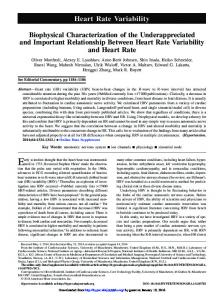
Chart I shows the annual rate of growth fot two-quarter periods and the longer-term trend rate of expansion (five years) since 1953. Economic theojy and empirical evidence indicate that sharp swings in the two-quarter growth rate of the money stock temporarily affect the growth i-ate of output and employment. The shaded areas in the chart, which indicate periods of business recession, are associated with relatively shatp slowings in short-run money growth relative to the trend growth i-ate.

Chart 1 also shows that the ~“rations of money growth about trend have been unusually wide since

FEDERAL RESERVE BANK OF ST. LOUIS

NOVEMBER 1984

Chart 2

Standard Deviations of Quarterly Ml Growth Percent

Percent

9

9

I

I

8

$

7

7

Four-quarter a

6

I

I

i

~

5

--—--~

6

t

I-—---

I

St I

5

-——

it

4

4

3

i~ ~

‘‘ ——-~—~

Vt Twent-quarterLZ

jl

‘.i

l

I

v,__~

‘I

‘t/il

~

It 3

‘I

~

;

I

H

2

2

—~4---y— II 45

¶JI

0

1954

,_._

J

IS

V

,

II

I ,

~

56

58

60

62

:

I It

i,>., ~ ~

64

I

~j~:

t

I ~ ,

66

68

I

c~ >_~ ____q______~ I • 5I_I 4~ —‘ j/

10

72

74

76

—

~

78

80

82

1984

0

Four-quarter standard deviation of Ml growth I400AInI> ~ Twenty-quarter standard deviation of Ml growth (400Aln).

1979. Statistical measures of money growth variability strongly support this visual evidence. Chart 2 shows the standard deviations for the growth rate of the quarterly money stock measured over the most recent four and 20 quarters since 1953. Both measures show relatively high levels of volatility since l979.~ 4

There are several reasons for increased variability of money growth since 1979> For example, Weintraub (1980), Tatom (1982), Hem (1982) and Board of Governors of the Federal Reserve System (1981) emphasize the effect of the credit control program on the currency ratio and, hence, on the link between reserves and monetaiy aggregates in mid—i 980. This factor contributed to the rise in the variability of money growth in 1980. Others have emphasized problems associated with financial innovations, especially late in 1982 and early in 1983, that led to the temporary abandonment of Mi targeting in October 1982.

The Variability of Interest Rates The variability of expected returns affects decisions because it influences the variability of wealth (the present value of expected income streams). For example, the present value of i-cal income expressed as a peipetuity is inversely proportional to the expected yield. That is, wealth (WI is the flow of income pci-year (VI discounted by the i-ate of interest paid on a perpetuity(i),W = V/i. Wealth holders are concerned with the likelihood of percentage variations in interest rates rather- than absolute percentage point changes. The wealth effect of

a 100 basis-point change in the expected interest rate is greater when the expected interest rate is 3 percent

33

FEDERAL RESERVE BANK OF ST. LOUIS than when it is 15 percent. In the former case, wealth can change by about one-thiid; in the latter case, wealth changes by about 6 percent. If risk is measuied relative to the expected return, the variability of ieturns should be measured relative to the mean return. The logarithm of the interest i-ate provides such a

mean-adjusted measure. The variability of the logarithm of wealth is directly related to the variability of the logarithm of the expected yield.’ Risk is measured here using the yield on Aaa bonds, since it is the longterm yield that is most important for capital accumu-

lation and has the greatest impact on wealth. The expected volatility of rates ofreturn is an impor-

tant determinant of investment decisions. It is not possible, however, to directly measure this risk.’ If assessments of this risk are reflected in the actual variability ofyields, then the variability of interest rates

in the recent past can be used as an indicator of risk. Even then, the length of the relevant past is essentially an empirical issue. Chart 3 shows the standard deviation of the logarithm of the quarterly Aaa bond yield, measured for the four and 20 quarters ending in each quartei shown, respectively, for the period from 1924 to 1983> These measures summarize the riskiness of yields during the respective past period. Both measures indicate a sharp jump to record levels in the variability of interest rates after 1979> In 1984, the 20-quarter measure declined sharply from its peak in early 1982, but it

remained near previous peaks achieved in the mid1930s, early 1960s and earl 1970s.

Other Measures of Interest Rate Variability There are a variety of other ways to measure the variability of interest iates> For example, Evans (1984) uses the standard deviation of monthly interest rate changes over a one-year period. ‘Fhe list of standard deviation measuies examined for this article includes,

‘Given expected income, (V), wealth is W” Y/i and the logarithm (In) of wealth is In V — In i. Thus, In W is inversely related to In i and the variance of In W is proportional to the variance of In i. Note also that the variance of (In i) is independent of the level of the interest rate since Var [In (k UI Var (In i), where k is a scalar multiple. ‘It would be most useful to measure the variability of the expected after-tax real rate of return and that of the expected rate of inflation separately. Makmn and Tanzi (1983) argue that an increase in both factors account for the increased volatility of interest rates in 1980— 82. Since both have qualitatively the same effect on investment, production and money demand incentives. the distinction is ignored here.

34

NOVEMBER 1984 besides the two measures in chart 3, the standard deviations of: the level of the quartei-ly interest rate, the change in the quai-terly interest i-ate and the change in the logaiithm of the quarterly interest i-ate. To test the effects of variability on economic perfoi-mance, each standard deviation measure, as well as the logarithm of each measure, was used. Two other measures were examined as well: the average absolute change in the level of the quarteily inteiest i-ate and the coefficient of variation of the quar-terly interest rate. All measures were computed for four-, 12- and 20-quarter periods> The best results (judged by robustness across perods of time and relative explanatory power for economic performancet were found using the 20-quarter standard deviation of the logarithm of the interest i-ate; this measure is called VII here. Virtually the same results are obtained using the 20-quarter- coefficient of variation, which is simply an alternative way of adjusting the variability of the intei-est rate for different mean levels over time. As emphasized above, it is such mean-adjusted measures of variability that, in principle, should matter. Othei- measures generally do not have significant economic effects; in those cases where significant economic effects al-c observed, relationships usually are either not robust or are statistically inferior in terms of explanatory power. These exceptions are noted below. Interest rate variability measures inherently depend on past interest rates. For example, a i-ise or fall in interest rates from one level that has persisted for a considerable time to another that will persist for a long time to come, will lead to a transitory rise in the

variability of interest rates during the ti-ansition fiom the former to the latter and for some period subsequently. The Aaa bond yield has broadly followed a pattern of three level shifts fi-om 1955 to 1983; it iose fiom about 3 percent dunng 1950—55 to neal- 4>5 percent during 1960—65, then rose to about 8 percent from 1970 to early 1977, and finally surged upward to an average of 13 percent in 1980—83> The three major spikes for the 20-quarter measure in chart 3 are consistent with such level shifts in interest rates. There are two ways to interpret this rise in variability. One way would suggest that the rise is

purely arithmetic with no economic consequences for perceived investment risk. The alternative view is that the rise in interest rate variability associated with such level shifts in interest rates mirrors the increased risk perceived from such unfoieseen changes> Moreover, this risk, like the variability measure, is reduced slowly over time> This aiticle assumes that the second inter-

FEDERAL RESERVE BANK OF St LOUIS

NOVEMBER 1994

Chart 3

Standard Deviations of the Logarithm of the Quarterly Average Aaa Bond Yield Percent 24

Percent 24

20

20

16

I’

12

12

8

8

4

4

0

192628 30 32 34 36 38 40 42 44 46 4$ 50 52 54 56 5$ 6062 64 66 68 10 12 14 76 78 80 $21984

pretation is more accurately descriptive of risk perceptions following such level shifts in interest rates.

The Link Between Variable Money Growth and Variable Interest Rates

0

Lags of the 20-quarter standard deviation of quarterly money growth shown in chart 2, VM, were introduced to test whether money growth variability influences interest rate variability, VR. The iesults foi the period 1/1955—IV/1983 are shown in table 1.

Both measures of the variability of money growth

There is a significant positive link between a rise in

shown in chart 2 rose shaiply beginning in 1980 and

the variability of money growth and the variability of

remained well above their previous average during

interest rates.’ When one contiols for the past two

1980—83. The variability of interest rates rose similarly, as chart 3 shows. An empirical investigation of the link between the variability of money growth and that of interest rates was conducted for the 20-quarter standard deviation measures shown in charts 2 and 3>’

quarters of the variability of interest 1-ates (longer lags

‘The best univariant time series model for VA is a second-order autoregressive and second-order moving average process during the periods I/i 955—l V/I 978 and I/i 955—IV/i 983>

‘These tests, including past information on interest rate and money growth variability, use the Granger causality test specification> However, unidirectional causality is not asserted, necessary, or tested here> Also, interest rate variability may be a function of other sources of increased risk including increased variability of fiscal policy variables. The importance of other factors is apparent over the 1955 to 1978 period, when VA showed considerable variation, but VM was essentially unchanged. 35

FEDERAL RESERVE BANK OF ST. LOUIS

ai-e not signiflcant( and for statistically significant second-order autocor-relation, the variability of mone growth over the previous two quarters has significant effects on the current level of the variability of interest ‘-ates.’ A rise in money growth variability initially has a significant arid positive effect on interest rate variability; this effect is offset in the next quarter.” According to table 1, the significant positive effect of the variability of money growth on interest rate var ability is transitory.” Attempts to replicate the table I results from t/1955— IV/1978 were unsuccessful; the variability of money growth did not significantly affect the variability of interest r-ates over this earlier period. A prncipal rca-

‘The 0-statistic indicates that the residuals in the equation estimate are not significantly correlated with their own past for up to 12 past quarters, although the same results holds for one to 24 past values of the residuals> “The results do not arise from the computational relationship arising from the use of moving standard deviations. Virtually identical results are obtained by relating changes in VA to aVR,~,,VA,,, and either VM,., and VM,,, or ,SVM,~,.First-differences of VM or VA are not computationally related. “The steady-state response of VA to a rise in VM involves the lagged adjustment of VA to its own past values> This response is 1>52, but its standard error, found from the variance-covariance structure of the coefficients on the lags of VM and VA, is 2.00. Thus, the effect of a change in VM is transitory. Whether a rise in money growth variability, in theory, has a permanent or transitory effect on interest rate variability is a question that is not resolved here> The empirical evidence cleariy indicates that the effect is transitory>

36

NOVEMBER 1984

son for this result is that the variability of money growth over- the period t/1955—IlI/1979 was relatively constant; the standard deviation of VM over this period is 0>3 percent, only 15>3 percent of the mean level of money growth vanability over the period. The variability of money growth from 1955 to 1979 was too small and steady to provide intbr-mation on the potential impact of changes in money growth variability on interest rate variability.”

Earlier Evidence: 1924 to 1954 Prior evidence of a systematic relationship between the vaiiability of money growth and interest rates does exist, however> Ftiedman and Schwaitz (1963( have shown that mone growth variability was much greater before World War II than it was from the end of World War II to the early 1960s.L The variability of money growth also fluctuated much more before World War II. The average level of VM from t/1924->-lV/ 1954 is 7.5 percent, and its standard deviation is 3 percent; the former is more than three times as large,

2 ‘ The mean of àVM from I/i 955—111/1979 is 0>0021 and its standard deviation is 0>1101> Over this period, iIVM is an independently distributed random variable with a 0-statistic, 0(12), of 7.34, which indicates that AXVM is not correlated with its past history. Over the longer period to IV/1 983, SVM is described by a first-order moving 1 average process. “Friedman and Schwartz (1963, pp. 592—638)> Their Ml data until 1947 is used to compute VM below>

FEDERAL RESERVE BANK OF ST. LOUIS and the latter’ measure is about 10 times as large as that observed fiorn 1955 to 1979. Thus, this eatlier period should provide useful information on the elfect of monetary growth variability on interest rate variability. Over the perod tll/1924—lV/1954, there is a statistically significant positive relationship between VR and VM (see table II. The results are similar to those for the 1955—83 period> In par-ticular, for this earlier perod, increases in the volatility of money growth temporarily and significantly raised the volatility of interest rates. Autocon-elated errors are not significant in the earlier period accor-ding to the Q-statistic> The dynamic structure for interest rate volatility is about the same as in the later’ period.” The difference in the magnitude of the money growth variability effect in the two periods is not meaningful; the money stock data used in the early period are lamgely based on endof-month data, while those in the later period are based on averages of daily figures>

VARIABILITY OF MONEY GROWTH AND INTEREST HATES’ THE AGGREGATE DEMAND CHANNELS Mascaro and Meltzer (1984) have attributed part of the substantial jump in interest rates and the decline in real GNP growth in 1980—81 to the increased uncertainty arising from greater- variability of money growth> They attribute a 1.3 percentage-point rise in the average long rate and a 3>3 percentage-point rise in the aver-age short rate over the nine quarter-s, IV/1979—lV/ 1981, to a rise in monetary uncertainty>’ Mascar-o and Meltzer emphasize a money demand channel for the effect of monetary uncertainty on the economy-A rise in monetary uncertainty increases the demand for’ money> They indicate that an incr-ease in the demand for money r-aises the interest rate and reduces aggregate demand. In addition, they argue, prices and real output fall because of the reduction in aggregate demand> Further-more, they suggest that the growth rates of output, prices and GNP are likely to be fur-ther affected by the reduced demand for- capital. Their empirical analysis focuses on the rise in inter-est r-ates on both shor-t- and long-term debt due to the risk premium>’ ‘~Overthis period, the t-statistic forthe steady-state response of VA to VM is 0>12; the response of VA to VM is transitory> “Belongia has argued that nominal GNP growth was depressed by the rise in monetary uncertainty in 1980> Both Mascaro and Meltzer and Belongia use a measure of the variability of unanticipated money growth rather than that of actual money growth>

NOVEMBER 1984 There is a second demand channel, however, through which money gr-owth variability lowers investment> When money growth is more variable, the variability of the output of goods and services, employment and earnings will rise. Ther-e will also be greater risk associated with the expected returns from both existing capital and prospective investments> If stockholders and lenders are risk averse, and if existing expansion plans and sources of financing are to be maintained mat-ket r-ates of retur-n must rise to compensate for increased risk> Of course, with higher- costs of capital funds and greater- risk associated with pr-nspective investment projects, investment managers will both reduce investment and enhance the flexibility of their asset portfolios.” Thus, because it contributes to more volatile investment returns, erratic money growth raises the level of observed market rates and retards and redirects the desired stocks and usage of plant and equipment. At unchanged interest rates and costs of funds for firms, a rise in the variance of expected returns from investment in plant and equipment reduces the incentive to invest. The portfolio shifts emphasized by Mascaro and Meltzer, and Gertler and Gr-inols (1982), involve an increase in money demand that raises interest r-ates> Investment demand in their analysis declines along a given investment demand curveS. But even at an unchanged cost of capital. fir-ms faced with riskier expected incomes will reduce investment.

“Bodie, Kane and McDonald (1983) find evidence of a rise in the risk premium on long-term bonds> Gertler and Grinols (1982) show that a rise in monetary growth uncertainty raises money demand and reduces investment, but their result follows primarily from an increase in the variability of expected inflation, not from an increase in the variability of the real rate of interest> If variations in money growth affect real output and employment in the short run, as monetary explanations of the business cycle indicate, then monetary randomness also affects the variability of the expected real rate and investment incentives, Indeed, this is more likely if the link between money and prices has long lags as shown in the model used below or in Barro (1981)> A rise in monetary variability raises the variability of yields on capital and reduces investment, either through increased variability of expected inflation or of real rates of return (both of which are captured in the variability of nominal interest rates), or both> Makin and Tanzi attribute the high volatility of interest rates from 1980 to the end of 1982 to increased volatility of both expected inflation and after-tax real rates of return. Their evidence for the former, however, is surveydata on expected inflation for a six-month horizon during a period in which substantial price level shocks were occurring> “Obviously a rise in risk tends to reduce both the supply of saving and investment demand at given market interest rates> Thus, the effect on observed market rates is not as straightforward as it may appear in the text> If suppliers of credit are more risk averse than firms that invest in plant and equipment, then market rates (not risk-adjusted) will tend to rise. This result also depends on relative interest elasticities of supplies and demands for credit and equities> 37

FEDERAL RESERVE BANK OF ST. LOUIS

Such a decline in the demand for goods and services is accompanied by a reduction in the demand for credit, so that interest rates tend to fall along with aggregate demand. The left side of figure 1 summarizes the two aggregate demand channels> These effects arise in this instance through increased money growth variability. Other changes that raise risk assessments about fu-

38

NOVEMBER 1984

ture economic conditions or business cycle risk could alter interest variability as well, however. There appear, then, to be at least two channels through which monetary gr-owth variability affects aggr-egate demand: increased money demand and reduced investment. Of course, the two channels have opposite implications for interest rates; both, however’, imply reduced aggregate demand and, hence, lower nominal GNP, real output and prices. The Mascar-o-Meltzer evidence on

FEDERAL RESERVE BANK OF ST. LOUIS

NOVEMBER 1984

interest rates suggests that the rise in money demand dominates risk-related reductions in the demand for goods and services. Figure 2

Evans (1984( and Tatom (1984a( show that a rise in the variability of interest rates has a significant negative effect on the level of annual output. ‘this effect is consistent with the two aggregate demand channels shown on the left side of figur-e 1, but it encompasses other sources of a rise in such variability besides a rise in monetary variability. To the extent that such variability arises from monetary variability, it simply reflects the channels through which money growth variability affects the levels of interest rates, spending, output and prices.

The Effect of arr Increase in Risk on Output and Price

VARIABILITY OF INTEREST HATES AND MONEY GROWTH: AGGREGATE SUPPLY A rise in risk implies, at the producer- level, incr-eased variability of expected sales, real cash flows or profits. A rise in the variability of r-eturns to production may be viewed as either- an increased cost of using the

Y

2

Yr

Yo

Rein ovtpvf

firm’s capital to produce output or a reduction in the value of given expected income. In either- case, exposure to the increased risk can be lessened by reducing expected output, production and capital employment in production. Thus, an increaèe in risk reduces desired supply, given expected prices of inputs and output.” This effect is summarized in the third channel of influence shown in figure 1> Whether supply is reduced more than demand is not obvious. Thus, while the consequences of increased risk for spending and output are unambiguous, given the price level, the consequences for the price level are not. Figur-e 2 shows the effect of a rise in risk, VR, on aggregate demand and supply. Initially, the economy is assumed to operate at point A where, at price level P,, the quantities of goods and services demanded and

‘8De Vany and Saving (1983) provide a model of the firm in which

greater variability of demand will yield higher pecuniary prices, the substitution of inventory for plant and equipment at a given expected output rate to the extent the product is storable, and, a reduction in expected output relative to capacity> Such reductions in the en iciency of firms indicate an overall loss in economic capacity or, for a given stock of plant and equipment and employment, less expected output> The firm in their model can be risk-neutral> Sandmo (1971) and Holthausen (1976) show that risk-averse firms reduce capacity and output in response to increased uncertainty, yielding similar price and output implications.

supplied (y,) are equal. An increase in risk reduces aggregate demand to AD,; at (P,,, y,), market interest rates, which are implicit in AD and AD,, are higher than at (P,,, y,(. Aggregate supply is reduced as well, however. As drawn in figure 2, AS shifts Ieftwar’d more than AD, so the price level rises to P,> Thus, the economy operates at point B. Of course, the price outcome depends on the relative magnitude of the supply and demand shifts. Eariier studies of monetary uncertainty and interest rate variability have focused primarily on their effects on nominal and real GNP and on the inter’est rate. The common assumption appear’s to be that the effects on spending and output arise fiom an unanticipated shift in aggregate demand, so that the price level changes in the same direction as spending or output. The model used below to assess the effects of interest rate variability is a reduced-form model for- GNP, price and output growth that permits all three effects to be examined; this model is shown in table 2. In the model without interest rate variability, GNP growth depends on current and past growth rates of the money stock, cyclicall adjusted federal expenditures, energy prices and a strike variable.” Inflation

39

NOVEMBER 1984

FEDERAL RESERVE BANK OF ST. LOUIS

77~
The details for its construction are available upon request from the author. The coefficients for money and expenditure growth were estimated using a fourth-degree polynomial with head and tail constraints. The energy price coefficients were estimated using a third-degree polynomial and were constrained to sum to zero, This constraint cannot be rejected in either period.

~

“

/

.7

/

,,4,

‘7/

I i”

/77721

7’\’C’7:/~:4&4”,,7~N 7 4N

7,

7

*i~’Øisiáis*iwb4a’MS W 7

SE 7’

/

7,

N

~4”

N~

~

7”

,A’

’’i’’,’

‘‘ Fur-ther, none of the other coefficients in table 3 are affected when vii, is used and the standar-d error- of the estimates compare favor-ably> In the period ending in lV/1983, the standard error is 3.111; in the earlier period it is 2.886> The adjusted R’s ar-c the same as in table 3> Thus, the source of the interest rate variability effect in table 3 is anticipated variability>’~ The results indicate that the effect of interest rate variability on GNP growth since 1979 discussed below is the same whether the measure chosen is the actual past level of volatility, Vii,.,, or- contempor-aneous or lagged anticipated volatility yR or Vii,. I.

Some Problems with the GNP Estimates It should be noted that the interest rate variability measure, eithervR,., or- Vii,, enters the GNP equation in level form. Thus, a rise in the level of Vii permanently affects the growth rate of nominal GNP> Tests of additional lags, especially Vii,. and Vii,.,, respectively, indicate that they are insignificant> This result suggests that a permanent rise in the variability of interest rates reduces both the level of GNP in the short run and the growth rate of spending permanently> “The significance of yR in both periods indicates that, given past interest rates, VM significantly reduces ONP> When VM and its lags are added alone to the table 1 equations, however, they are not significant>

42

NOyEMBER 1984 The latter effect is theoretically implausible; the capital stock eventually should be adjusted to its lower desired level. Once this has occurred, the permanent effect on the growth of nominal spending and real output should disappear. The dynamic structure of Vii indicates, however, that interest rate volatility tends to revert to its mean following changes in money growth variability or random shocks. Thus, because changes in interest rate volatility are transitory, changes in the GNP growth rate arising from interest rate variability are transitory as well. A second concern with the GNP evidence is that variability measured over’ two shorter time horizons (four and 12 quarters) does not have a significant effect on GNP growth, nor do a few other measur-es of var-lability for- any horizon. There ar-c two ways to interpret the GNP results. One interpretation is that changes in interest rate variability ar-c only important when viewed from a longer’ time horizon and, even then, only certain measures of variability such as Vii, the coefficient of variation of the interest r-ate or’ aver-age absolute changes in the interest rate) capture the relevant risk. The other alternative is that the GNP results are spurious. The consistent results fl-nm the tests for prices below suggest that the latter inter-pretation is not valid>

The Effect of Interest Rate Variability on Prices The theoretical discussion indicates that the effect of increased interest rate variahility on prices is an empirical issue; it depends on whether- aggregate supply is affected more or less than aggregate demand. To assess this r-elationship, a standard pr-ice equation which emphasizes the link between money gr-owth and prices, contr-olling for shocks such as wage and price controls and ener~’ pr-ice changes, is employed. The price equation used for- the test of an inter-est rate variability effect is the second equation in table 2!” Again, both permanent and tr-ansitorv effects of interest rate variability were examined> As with the GNP experiments, the five-year’ measure “The coefficients on money growth are estimated to lie along a thirddegree polynomial. “A 12-quarter measure of the standard deviation of the logarithm of the interest rate has a positive and statistically significant effect at one lag in the period ending in V/i 983, but the equation has a higher standard error than the same estimate using the 20-quarter variability measure. The 20- and 12-quarter average absolute change in the interest rate also significantly raises then lowers inflation at lags one and two, respectively, over the longer period, but no effect is significant in the earlier period> See also footnote 31 below>

FEDERAL RESERVE BANK OF ST. LOUIS

V

NOVEMBER 1984

~tt

~

~,

7

,~

.7

~ ~7

//

7

~

~

/~‘//

~

#i~7 /,/~/ :/< ~/~7t/ 7 /~

——

///

//~/~

/_

/

/

//

>A~

~/

\

/

c00 in the I/1955—IV/1983 period. “This result is at odds with that found using annual data where interest rate variabilityappears to have a permanent positive impact on the price level. See Tatom (1984a)> It is shown below, however, that a distinction between anticipated and unanticipated variability yields results that are consistent with the annual result tor the price level,

‘S.,

/

the price level are unaffected.zT The sum of the coefficients on the change in interest rate variability in table 4 is positive, but not significantly different fl-nm zeni tn the L’1955—IV/1978 period, the sum is 0>130 It = 0.62), while in the 1/1955—IV/1983 period it is 0.283 It = 1.27).’~ The anticipated/unanticipated variability distinction was also employed to isolate the inflation effect. When Vii,,,,, Vii,,,, and Vii,.., are decomposed into anticipated and unanticipated components using the table I equation, only the lagged unanticipated component,

‘~Theprice equation is stable across the two periods in table 4. The F-statistic for the last 20 observations is F,,,e 1 .66, which is below the critical value of I .69 (5 percent significance level). The equation is not stable without the interest rate variability term. See Tatoni (19Mb), where tests of other variables (such as shifts to other checkable deposits or unusual recent movements of exchange rates, the volatility of money growth, unemployment or interest rates) that might affect prices indicate that, since mid-i 981 , only unemployment and the previous quarter’s change in the In of the Aaa bond rate significantly affect the price level. The unemployment result does not hold before IV/l 981 and disappears even in the later period when the past interest rate change is included. The bond yield result is robust across the periods> When either of these variables is added to the estimates in table 4, however, it is not significant in either period, and the interest rate variability result is unaffected. This also indicates that controlling for the level of interest rates in table 4 does not affect the result there. 43

FEDERAL RESERVE BANK OF ST. LOUIS VRE,.,, is significant, and in both periods> Tests of lags of VRE or- Vii yielded the same conclusion for- VRE and indicated that both Vii, and Vii,., terms are statistically significant in both periods> tn addition, the coefficients on the two anticipated variability tei-ms can be constrained to sum to zero; in the t/1955—tV/ 1978 period, F,,- = 0.00, while in the longer period, F,,,,, = 0.70. The inflation equations with VRE,., or- AVii, ar-e given in table 5, along with the inflation equation containing both variables.29 The results do not discriminate between the alternative hypotheses that only anticipated )AvIU or- unanticipated VilE) interest r-ate variability matters in the t/1955—IV/1983 period. Either- specification yields the same adjusted ii’ and standard error ofestimate; when one ofthese variables is included, the other is not significant. In the ear-her period, however, lagged unanticipated volatility slightly outper-forms the anticipated variability specification. Moreover-, the tests show that when ViiE,, is included, information on anticipated vanability is not statistically significant. The effect of interest r-ate volatility on prices is unambiguous, according to the results in table 5. tn particular-, a rise in anticipated variability temporarily raises inflation, leaving the price level unambiguously higher. Although it may appear that a rise in unanticipated var-lability permanently r-aises prices and inflation, only the former conclusion is correct; this result is the same as that obtained when only anticipated inflation is consider’ed. A rise in the unanticipated variability of inter-est rates cannot permanently raise inflation because, by definition, the level of unanticipated variability is only a transitory phenomenon. The evidence supports the dominant supply-side

“In table 4, the included lags of VA can be written as (VA,, VR,.,, VA,.,, VA,.,), where the coefficient on VA, is constrained to zero. A more general specification includes the anticipated (VA) and unanticipated component (VAE) of each of the VA effects above, where these components at each lag are not constrained to be equal. From this specification, the constraints involved in table 5 can be tested apd found to hold. These constraints are that the coefficients on VR,,, VRE,,,, VA,.,, VAE,,,, and VRE, are zero; and they hold when tested jointly or separately> One cannot discriminate statistically between the hypotheses that the coefficients on VA and VA,., are significantly different from zero and opposite in sign1 while that on VAE,., is zero and the hypotheses that the coefficient on VAE,,, is significantly different from zero and those on VA, and VA,,, equal zero. An implication of these results is that the apparent insignificance of VA, in table 4 arises from the imposition of the unsupportable constraint that the effects of VA, and VAE, are the same. Thus, the following constraints in table 4 do not hold: that the coefficient on VA, is zero or that the coefficients on VA,., equals that on VAE,.,. When these constraints are relaxed, both components of VA,,, and VA,., drop out. 44

NOVEMBER 1984 effect of inter-est r-ate variability: a r-ise in inter’est i-ate vai-iability unambiguously raises pr-ices permanently, thr-ough ‘a tempor-ar~ rise in inflation, hut it has no permanent effect on the inflation rate> The evidence, however, does not discr’iminate well between whether the permanent effect on prices arises fl-nm changes in anticipated variability or past unanticipated variability.

The Effect of Interest Rate Variability on Output The gr-owth rate of i-cal GNP in the model in table 2 equals the difference between the gr-owth r-ate of GNP and the gr-owth rate of pr-ices; it can be written as the right-hand-side of the GNP equation less the righthand-side of the price equation. Consequently, the effect of interest r-ate volatility on output gr-owth is the difference in the Vii components in the appr-opriate GNP and price equations. Since a permanent rise in interest r’ate variability permanently lowers the gi-owth rate of GNP and temporarily raises the inflation r-ate, the per-manent effects on i-cal output and its gr-owth rate are unambiguously negative. An estimate of the effect of interest rate variability on output growth is found using the actual variability results in tables 3 and 4. For’ the t/1955—IV/1983 period, the output growth effect is (—1.572 S vii,,, + 0.654 A yR. — 0.297 Vii,.:,); t-statistics for- the three coefficients are —5.76, 2.42 and —4.87, r-espectively. When the anticipated interest rate variability measure results are combined, the r’eal GNP growth r-ate effect is —0.937 AVR, — 0,289 Vii,.,); the t-statistics for the two coefficients are —5.78 and —4.75, respectively. The longrun effect on the real GNP growth rate indicated by the last term is essentially identical for both specifications, while the timing and short-r-un effects are slightly different. Of cour-se, the same effects can be estimated using the unanticipated volatility effect on prices and the anticipated volatility effect on GNP; when this is done, once again, the differ-ences are slight.

The Estimated Effects on Economic Performance: 1980—83 To gain some insight into the magnitude of the estimated effects above, the actual levels of Vii, fr-nm 1/1980 to IV/1983 are given in table 6, along with the effects on the growth rates of GNP, prices and real GNP, due to the departure of Vii from its I/1955—III/1979 mean level of 8.60 percent> The effects for GNP, prices and output

FEDERAL RESERVE BANK OF ST. LOUIS

NOVEMBER 1984

45

V FEDERAL RESERVE BANK OF ST. LOUIS

/

NOVEMBER 1984

:,

\

\j

/

/

~.

~tb’~~

..

~,

~

~~iç

/t

\

~

.

C~’i>

~

//~

‘~

~

/‘~

*~PV’ ~

/

~

::‘

‘~

/ ~,,

~

~

/

~

\

:~

. ~

~

~

/4~/4~:~~ ~.c ‘V%,~

-a

~

~

~ :: :~.

~ “

N~>.

4t~e~:V t\.\~~V~’

x~

.~\

~

~

/:

,

—

.

~

~

~V

in table 6 use the l/1955—IV/1983 estimates of the impact ofanticipated variability reported above. The estimates based on actual or unanticipated variability effects are about the same for- the whole period or for subperiods such as the 1981—82 recession. Changes in risk, as measured by the five-year standar-d deviation of the logar-ithm of Aaa bond yields have had a substantial impact on the economy since 1979, generally retarding the growth r’ate of nominal and real GNP over the period. In 1980—81, the rise in risk temporarily raised the observed inflation rate. The subsequent fall in risk temporarily reduced inflation in 1982—83. Table 6 indicates that greater interest rate variability reduced the growth rates of nominal spending and real GNP by an average of 2.3 and 3.8 percentage

“Evans also reaches this conclusion. Using the estimates based on actual variability, the reduction in nominal GNP over the whore period shown in table 6 is 2.7 percentage points, while during the recession it is 3>9 percentage points; the reduction in real GNP growth over the whole period is 2>8 percentage points and 3.6 percentagepoints during the recession> Similar estimates are found using the unanticipated interest rate variability hypothesis for prices; real output falls 2.6 percentagepoints over the whole period and 3>7 percent during the recession.

46

,

.~.ct ~

~ç[~:

‘

~

\

/

4V’

/‘/\

~

\

~

/

.

~

~

—/~,

(

‘~

~

.\~

V~ /)~\

~

‘

‘~/

~

/

,.

~

‘2

,

~

~

~

\

/

~

/

\~/

/

~

~ \~*$~

,

points, respectively, during the ILI/1981—IV/1982 recession.” Thus, such variability played a major role in the relatively sluggish growth ofspending at a 2.8 percent rate over the period and the —2.4 percent growth rate of real GNP from peak to trough> tndeed, departures from the mean variability had a negative impact on real output growth that exceeds the observed decline, suggesting that, in the absence ofincreased variability, real GNP growth would have been positive>”

“When the measure of variability is the 20-quarter standard deviation of the changes in the logarithm of the quarterly interest rate, similar significant effects are obtained for GNP, prices and real GNP. Over the period l/1955—IV!1983, the current and past four levels of this standard deviation measure significantly affect GNP growth. The sum effect is significantly negative> In the price equation, only the change in the standard deviation three quarters earlier is significant. For both equations, the statistical results are inferior to those presented in the text, judged by the fit of the equations. Also, the results are not as robust> In the I/I 955—lV/1 978 period, no lag of this measure adds significantly to the price equation; in the GNP equalion, only the lagged change in the standard deviation approaches significance (t = —1 >92)> The quantitative effects of higher variability on ONE. prices and output using this measure, however, are similar to those found from tables 3 and 4 or those given in table 6> For example, over the recession period IlI!1981—lV/1982, nominal and real GNP growth were reduced by an average 2>7 percent, while inflation was unaffected. The anticipated/unanticipated variability tests were not conducted for this measure due to the inferiority of the actual variability results>

Fcuc~LRESERVE BANK OF ST- LOUIS

SUMMARY AND IMPLICATiONS The evidence here generally supports recent studies which indicate that increased variability of money stock growth and interest rates in the early 1980s had deleterious effects on output and employment. Moreover, the evidence provides a link between the rise in money growth and interest rate variability. The rise in the variability of interest rates, in particular anticipated variability, was an important channel through which increased monetary uncertainty operated to reduce GNP, output and employment, and to first raise, then lower, inflation alter 1979. The empirical results suggest that the rise in interest rate variability after 1.979 explains the severity of the 1981—82 recession. The results also shed some light on the magnitude of the swing in observed inflation from 1980—81 to 1982—83. Inflation was first pushed up temporarily in 1980—81, then down in 1982—83 due to the pattern of changes in interest rate volatility since 1979.

REFERENCES Barro, Robert J. Money, Expectations and the Business Cyc/e (Academic Press, 1981). Batten, Dallas S., and Courtenay C> Stone> “Are Monetarists an Endangered Species?” this Review (May 1963), pp. 5—16. Belongia, Michael T. “Money Growth Variability and GNP,” this Review (April 1984), pp. 23—31> Board of Governors of the Federal Reserve System, Federal Reserve Staff Study, New Monetary Control Procedures (February 1981). Bodie, Zvi, Alex Kane, and Robert McDonald. “Why Are Real Interest Rates So High?’ National Bureau of Economic Research Working Paper #1141, (June 1983)> Bomhoff, Edward J> Monetary Uncertainty (Elsevier Science Publishers B.V>, 1983). Carlson, Keith A> “A Monetary Analysis of the Administration’s Budget and Economic Projections,” this Review (May 1982), pp. 3—14> De Vany, Arthur S., and Thomas A> Saving> “The Economics of Quality,” Journal of Political Economy (December 1983), pp. 979— 1000> Evans, Paul> “The Effects on Output of Money Growth and Interest Rate Volatility in the United States,” Journal of Political Economy (April 1984), pp. 204—22> Friedman, Milton> “What Could Reasonably Have Been Expected From Monetarism: The United States,>’ presented to The Mont Pelerin Society, 1983 Regional Meeting, Vancouver, Canada, August 1983,

NOVE~aWER1984 and Anna Jacobson Schwartz. A Monetary History ofthe United States, 1667—1960 (Princeton University Press, 1963).

________

Gertler, Mark, and Earl Grinots> “Monetary Randomness and Investment,” Journal of Monetary Economics (September 1982), pp. 239—58. Gilbert, R. Alton, and Michael E> Trebing> ‘The FOMC in 1980: A Year of Reserve Targeting,” this Review (August 1981), pp. 2—I6> Hem, Scott E> “Short-Run Money Growth Volatility: Evidence of Misbehaving Money Demand?” this Review (June/July 1982), pp. 27—36. Holthausen, Duncan M> “Input Choices and Uncertain Demand,” Anedcan Economic Review (March 1976), pp. 94—103> Lang, Richard W. “The FOMC in 1979: Introducing Reserve Targeting,” this Review (March 1980), pp. 2—25> Makin, John H. and Vito Tanzi, “The Level and Volatility of Interest Rates in the United States: The Role of Expected lntlation, Real Rates, and Taxes,” National Bureau of Economic Research Working Paper#f 167, (July t983)> Mascaro, Angelo, and Allan H> Meltzer> “Long- and Short-Term Interest Rates in a Risky World,” Journal of Monetary Economics (November 1983), pp. 485—518. Sandmo, Agnar. ‘On the Theory of the Competitive Firm Under Price Uncertainty,” Nnerican Economic Review (March 1971), pp. 65—73. Tatom, John A> “Interest Rate Variability and Output, Further Evidence,” Federal Reserve Bank of St. Louis Working Paper #84016 (July 1984a). ______“A Review of the Performance of a Reduced-Form Monetarist Model,” Federal Reserve Bank of St. Louis Working Paper #84-015 (July 1984b)> ________ “Alternative Explanations of the 1982—83 Decline in Velocity,” in Monetary Targeting and Velocity (Federal Reserve Bank of San Francisco, 1983), pp. 22—56> “Recent Financial Innovations: Have They Distorted the Meaning of Ml?” this Review (May 1982), pp. 23—35> “Energy Prices and Short-Run Economic Performance,” this Review (January 1981), pp. 3—17> “Does the Stage of the Business Cycle Affect the Infla lion Rate?” this Review (October 1978), pp. 7—15> Thornton. Daniel L. “The FOMC in 1982: Deemphasizing Ml,” thi Review (June/July 1983), pp. 26—35> Wallich, Henry C> “Recent Techniques of Monetary Policy,” Feder. Reserve Bank ot Kansas City Economic Review (May 1984), p 21—31> Walsh, Carl E> “Interest Rate Volatility and Monetary Policy,” Jt~ na/of Money, Cred/t and Banking (May 1984), pp. 133-50> Weintraub, Robert. ‘The Impact of the Federal Reserve Syster Monetary Policies on the Nation’s Economy” (Second Repo Staff Report of the Subcommittee on Domestic Monetary Policl the Committee on Banking, Finance and Urban Affairs, Housr Representatives, 96 Cong., 2 Sess>, (Government Printing Off December 1980)>