Based on the continuous Boltzmann equation with appropriate .... the CarnahanâStarling fluid [20] which equation of state leads to the following Ï: Ï = ÏRT.
Computer Physics Communications 129 (2000) 121–130 www.elsevier.nl/locate/cpc
Interface and surface tension in incompressible lattice Boltzmann multiphase model Raoyang Zhang ∗ , Xiaoyi He, Shiyi Chen Theoretical Division and the Center for Nonlinear Studies, Los Alamos National Laboratory, Los Alamos, NM 87545, USA
Abstract This paper studies the interfacial dynamics and surface tension in an incompressible lattice Boltzmann multiphase model proposed recently by He et al. [J. Comput. Phys. 152 (1999) 642]. The model tracks different phases and the interface between them using an index fluid with molecular interaction. When the molecular interaction is strong enough, the index fluid automatically segregates into two different phases. The surface tension is implemented in the model using a term as a function of the gradient of the index fluid density. The strength of the surface tension depends on the molecular interaction, and can be adjusted conveniently by a free parameter. Numerical simulations for a variety of flow conditions with surface tension are carried out to demonstrate the capability of the model. 2000 Published by Elsevier Science B.V. All rights reserved.
1. Introduction Surface-tension-involved multiphase flow is ubiquitous. The understanding of multiphase flows is of great significance for both fundamental research and engineering applications. The complexity due to interface deformation and interaction poses a formidable task for theoretical and experimental approaches, even though they do have provided perceptive insights to some of its basic characteristics [2]. The recent development of the computer technology and computational methods makes the numerical simulation a useful tool for studying the underlying physics of this phenomenon. Using the lattice Boltzmann method (LBM) to study multiphase flow has attracted much attention in recent years [3]. The unique feature of the LBM is its kinetic and dynamic nature. Residing on a mesoscopic level, LBM simulates fluid flow by tracking evolutions of the distribution function of assembly of molecules. In doing so, LBM is able to incorporate the intermolecular interaction which is the physical origin of phase segregation and surface tension. The interfacial dynamics, which is essential for multiphase flow but difficult to deal with at the macroscopic level, can be readily modeled in LBM by incorporating the intermolecular interaction. In addition, LBM is computationally more efficient than molecular dynamics, by avoiding tracking individual molecules. There have been a number of multiphase LBM models proposed in literature. Among them are the mutually repulsive two-color particle models [4–6], the inter-particle potential model [7–9], and the free-energy model [10– 12]. Each of these models has been successfully used to study certain multiphase flow phenomena (for review, see ∗ Corresponding author.
0010-4655/00/$ – see front matter 2000 Published by Elsevier Science B.V. All rights reserved. PII: S 0 0 1 0 - 4 6 5 5 ( 0 0 ) 0 0 0 9 9 - 0
122
R. Zhang et al. / Computer Physics Communications 129 (2000) 121–130
[3]). A recent study [13] shows that the lattice Boltzmann method for multiphase flow can be formulated based on the kinetic theory for dense fluids. Along this line, a new LBM model was proposed by He, Chen and Zhang for simulation of incompressible multiphase flows [1]. The incompressible LBM multiphase model by He et al. uses an index fluid to track different phases and the interface between them. It uses the molecular interaction to simulate phase separation and interfacial dynamics. When the molecular attraction is strong enough, the index fluid automatically segregates into two different phases. For a fluid that originally settles in two different phases, the molecular interaction keeps the different phases segregated. The interface between phases consequently remains sharp throughout simulations. This model has been used to study both two- and three-dimensional Rayleigh–Taylor instability without surface tension [1,14] and the simulations yield satisfactory results. The surface tension can be naturally incorporated in the new model using a forcing term which involves derivatives of the index fluid density. The theoretical framework for incorporating surface tension has been established in [1,14], but no benchmark study has been carried out. Since the surface tension and the interfacial dynamics are important in many multiphase applications, it is desirable to carry out detail studies on these issues. The rest of paper is organized as follows. Section 2 briefly describes the formulation of the incompressible LBM multiphase model proposed by He et al. Section 3 presents studies of the surface tension and numerical simulations of a variety of surface-tension related multiphase flow. Section 4 concludes this paper with a summary.
2. Theory The basic idea of the lattice Boltzmann multiphase model proposed by He et al. [1] is to use an index fluid to track the interface between two different phases which is similar to the level set approach [15]. Interfacial dynamics is simulated by incorporating molecular interaction. Based on the continuous Boltzmann equation with appropriate incompressible approximation, the evolution equations for both index distribution function and pressure distribution function can be derived to follow the interface and simulate the physical dynamics [1,14]. The primary variables used in the simulations are f¯, index distribution function, and g, ¯ pressure distribution function, which satisfy the following evolution equations: f¯α (x + eα δx , t + δt ) − f¯α (x, t) eq f¯α (x, t) − fα (x, t) (2τ − 1) (eα − u) · ∇ψ(φ) − Γα (u)δt , =− τ 2τ RT g¯α (x + eα δx , t + δt ) − g¯α (x, t) eq g¯α (x, t) − gα (x, t) =− τ � � 2τ − 1 (eα − u) · Γα (u)(Fs + G) − (Γα (u) − Γα (0))∇ψ(ρ) δt , + 2τ where δt is the time step which is usually taken as the time unit in LBM, G is the gravity force, and � � u2 eα · u (eα · u)2 + − . Γα (u) = wα 1 + RT 2(RT )2 2RT eq
(1)
(2)
(3)
eq
fα and gα are the corresponding equilibrium distributions: � � eα · u (eα · u)2 u2 eq + , − fα = wα φ 1 + RT 2RT 2(RT )2 �� � � u2 eα · u (eα · u)2 eq + , − gα = wα p + ρRT RT 2RT 2(RT )2
(4) (5)
R. Zhang et al. / Computer Physics Communications 129 (2000) 121–130
123
where R is the gas constant and T is the background temperature, and RT = 1/3 in our simulations. eα is the underlying lattice and for two-dimensional flow, we can use the following 9-speed model [17]: 0, α = 0, (α−1)π � (α−1)π �� cos , sin c, α = 1, 2, 3, 4, (6) eα = 2 2 � �� √ (α−5)π (α−5)π π π 2 cos + 4 , sin + 4 c, α = 5, 6, 7, 8. 2 2 √ Here c = 3RT and wα are the corresponding integral weights [16]: ( 4/9, α = 0, wα =
1/9, α = 1, 2, 3, 4, 1/36, α = 5, 6, 7, 8.
The density of the index fluid, φ, the pressure, p, and the velocity, u, are calculated using: X f¯α , φ= X 1 p= g¯ α − u · ∇ψ(ρ)δt , 2 X RT (Fs + G)δt . ρRT u = eα g¯α + 2 The real fluid density and the kinematic viscosity can be calculated from the index function using: φ − φl (ρh − ρl ), φh − φl φ − φl (νh − νl ), ν(φ) = νl + φh − φl
ρ(φ) = ρl +
(7)
(8) (9) (10)
(11) (12)
where ρl and ρh are densities of light fluid and heavy fluid, respectively; νl and νh are viscosities of the light fluid and the heavy fluid, respectively; φl and φh are the minimum and maximum values of the index function. φl and φh can be determined either theoretically by the equation of state or numerically. In our simulation, φl = 0.02381 and φh = 0.2508. Eq. (11) essentially is a linear mapping function between the index function φ and real density ρ. The function ψ(φ) in Eq. (1) plays a key role in multiphase flow simulations. The term ∇ψ(φ) is a mimic of the physical intermolecular interactions in non-ideal gases or dense fluids. Unlike those in an ideal gas, molecules in dense fluids experience attractions from neighboring molecules [18]. Collisions among molecules in dense fluids are also strongly affected by the density [19]. Using the mean-field approximation, these two effects can be incorporated into an effective force which determines the phase segregation [13]. In this study, we choose to use the Carnahan–Starling fluid [20] which equation of state leads to the following ψ: � � 1 + φ + φ2 − φ3 − 1 − aφ 2 , (13) ψ = φRT (1 − φ)3 where a determines the strength of molecular inter-attraction. The surface tension is implemented in the model through the term: Fs = κφ∇∇ 2 φ,
(14)
where κ determines the magnitude of the surface tension. The kinematic viscosity relates to the the relaxation time by ν = (τ − 0.5)δt RT . The corresponding macroscopic index equation for Eq. (1) and macroscopic dynamical equations for Eq. (2) are � � φ ∂φ + ∇ · (φu) = −λ∇ · ∇p(ρ) − ∇p(φ) , (15) ∂t ρ
124
R. Zhang et al. / Computer Physics Communications 129 (2000) 121–130
1 ∂p + ∇ · u = 0, ρRT ∂t � � ∂u + (u · ∇)u = −∇p + ∇ · Π + κφ∇∇ 2 φ + G. ρ ∂t
(16) (17)
Here all equations have the second order accuracy in both space and time. Eq. (15), which is similar to the level set function [15], tracks and separates different phases. And Eq. (17) describes the interested dynamics. In nearly incompressible limit, the time derivative of the pressure in Eq. (16) is small and the incompressible condition is approximately satisfied.
3. Results 3.1. Surface tension as a function of the molecular interaction According to previous theory [21], if we assume that the normal direction of the interface is along the z direction, the surface tension in the LBM multi-phase model can be written by an integration across the interface: Z � �2 ∂φ dz. (18) σ =κ ∂z Obviously, the surface tension depends on both parameter κ and the density profile across interface. In theory, the density profile is exclusively determined by equation of state and the parameter κ. In simulation, however, it also depends on the discretization scheme and needs be determined beforehand. Nevertheless, for a given parameter, a, and given numerical scheme, we can specify a surface tension by choosing: σ , κ= I (a) where
Z �
I (a) =
∂φ ∂z
�2 dz.
Fig. 1 shows the dependence of I on a for Carnahan–Starling fluid in our scheme. Also shown in the plot is the fitting curve: I (a) =
0.1518(a − ac )1.5 , 1 + 3.385(a − ac )0.5
(19)
where ac = 3.53374 is the critical value of Carnahan–Starling equation of state, below which a fluid can not separate into different phases. 3.2. Laplace law To study the surface tension, we investigate the pressure difference across the interface of a static bubble. Initially, a region with higher density is placed in the center of the lattice domain with 1282 resolution. When the system reaches equilibrium, a liquid bubble forms with a fine circular shape. According to the Laplace law, the pressure difference between the interior and the exterior of the droplet, 1P = Pin − Pout , is related to the surface tension, σ , via the following rule: σ (20) 1P = , R
R. Zhang et al. / Computer Physics Communications 129 (2000) 121–130
Fig. 1.
125
Fig. 2.
Fig. 1. The dependence of I on a. The diamonds are from the numerical result and the solid line is for the fitting curve. ac = 3.53374 is the critical value for phase separation. Fig. 2. The theoretical prediction (solid line) and numerical measurements of Laplace law. The diamond, cross and square signs represent the results of κ = 0.1, κ = 0.5 and κ = 1.0, respectively.
where R is the bubble radius. We conducted simulations for three different surface tensions with a = 4.0. Fig. 2 shows the measurements of 1P /κ versus 1/R, along with the analytic solution, Eq. (18). The diamonds, crosses and squares represent the results with κ = 0.1, κ = 0.5 and κ = 1.0, respectively. As shown, our simulation results stay very close to the theoretical prediction (solid line). The biggest error is less than 4%. The good agreement indicates the accuracy of the surface tension model in our LBM multiphase model. 3.3. Capillary wave As another interesting application, we compute the dispersion relation of the capillary wave between two fluids. An analytic solution exists for a sinusoidal long capillary wave with small perturbation. For simplicity, we assume both fluids have the same kinematic viscosity. The Atwood number, A = (ρh − ρl )/(ρh + ρl ), is fixed at 0.5. In the long wavelength limit, the decay rate and oscillating frequency are functions of A, surface tension σ and the wave number k of the initial perturbation. According to linear perturbation theory [22], the decay rate and the oscillating √ frequency, non-dimensionalized by k 3/2 σ/(ρh + ρl ), can be calculated as the real and imaginary parts of n=
y2 − 1 √ , s
(21)
where s = σ/k(ρh + ρl )ν 2 and y is the solution of the following quadratic equation: y 4 + 4α1 α2 y 3 + 2(1 − 6α1 α2 )y 2 − 4(1 − 3α1 α2 )y + (1 − 4α1 α2 ) + s = 0,
(22)
where α1 = ρh /(ρh + ρl ) and α2 = ρl /(ρh + ρl ). To study capillary wave, we carried out simulations on square domains with resolutions of 642 and 2562 , respectively. Period boundary condition is used horizontally and non-slip wall boundary is applied in the vertical direction. Initially a single sinusoidal wave is sitting in the middle of the domain with wavelength L equal to the domain size. The amplitude of the perturbation is set to be 5% of L to satisfy the condition of long wavelength limit. Fig. 3 is the comparison of our measurements with analytical solution. In the figure, the solid line is the theoretical prediction of the decay rate vs the non-dimensional parameter s, which stands for the ratio of the Reynolds number, Re = U L/ν, to the Capillary number Ca = 2πU µ/σ . The dashed line is the prediction of the
126
R. Zhang et al. / Computer Physics Communications 129 (2000) 121–130
Fig. 3. The theoretical prediction and numerical measurements of capillary wave dispersion. Solid line represents theoretical decay rate. Symbols represent numerical measurements of decay rate with different resolution: Circle (2562 ), and diamond (642 ). Dashed line represents theoretical oscillating frequency. Symbols represent numerical measurements of oscillating frequency with different resolution: fancy diamond (2562 ), and square (642 ).
oscillating frequency vs s. There exists a critical s0 ∼ 0.6 below which an initial perturbation decays without any oscillation. Our simulations reproduce this phenomenon quite well. With s larger than s0 , the oscillating frequency increases and the decay rate decreases with s. Although our simulation results of decay rate agree with the theoretical prediction quite well, where most of errors are less than 1%, the measured frequency is 6 ∼ 10% less than theoretical results. This systematic error seems not to change much for different numerical resolutions. There are several possible sources which may attribute to the discrepancy between the simulated frequency and theoretical prediction. First, the dynamic surface tension effect is more complicated than the static one. From the figure, we see that the influence of dynamic surface tension is smaller than theoretical prediction, although our measurement during oscillation still matches Eq. (18) well. Secondly, the average thickness of the surface interface is about 3 to 4 grid size. Thus, the linear interpolation defined in Eqs. (11) and (12) might not be accurate enough and may affect interfacial dynamics. Third, the numerical calculation of the third-order density gradient in Eq. (14) might not be accurate enough. The truncation error from numerical discretization can reduce the dynamic surface tension. Finally, the wall boundary condition applied in the vertical direction can also influence the accuracy of our numerical result. Nevertheless, this issue needs more studies in future. 3.4. Relaxation of droplet The third test case we studied is the relaxation of a deformed droplet driven by surface tension. The droplet initially has a square shape in the middle and semi-circle shapes at two ends. This initial shape resemble a droplet confined in a 2D channel. With a proper capillary number under threshold, the deformed droplet would slowly relax back to an equilibrium circular shape without oscillating. The simulation was carried out on a 1282 meshes. A finite element simulation with the same initial condition is conducted to check our result. The finite element analysis was carried out using the commercial computational fluid dynamics package, FIDAP (version 7.62, marketed by Fluent Inc.). The mesh convergence is verified by comparing results on a coarse mesh and a fine meshes. Fig. 4 shows the evolution of both the long and short axes. The solid lines are from the finite element results and the diamonds are from LBM results. Good agreement is observed. 3.5. RT instability with surface tension effect As the last benchmark study, we simulate Rayleigh–Taylor instability with surface tension to quantify the capillary effect on Rayleigh–Taylor instability. The capillary effect is usually characterized by Weber number
R. Zhang et al. / Computer Physics Communications 129 (2000) 121–130
Fig. 4.
127
Fig. 5.
Fig. 4. Comparison of axis evolutions vs time. Solid lines are from the finite element results. The diamonds are from LBM results. Fig. 5. Comparison of dependence of linear growth rate on its wave number and on the surface tension parameter S. Solid lines are from theoretical linear analysis. The diamonds are from LBM results. The lines from left to right represent the cases with S = 1.0, S = 0.5, and S = 0.0, respectively.
We = 2aρU 2 /σ or the capillary number Ca = µU/σ . When the capillary effect becomes important (We < 10), it stabilizes the interface and prevents the evolution of unstable structures. Fig. 5 shows the comparison of our simulation results with linear theory of the initial growth rates of RT instability. Similar to the dispersion case, the linear growth rate, non-dimensionalized by (g 2 /ν)1/3 , can be calculated as: n = (y 2 − 1)Q−2/3 , where
Q = g/k 3 ν 2 ,
Q−
(23)
g is gravity, and y is the solution of:
� y −1 Q1/3 S = y 3 + (1 + 4α1 α2 )y 2 + (3 − 8α1 α2 )y − (1 − 4α1 α2 ) , α1 − α2 α1 − α2
(24)
where S = σ/(ρl + ρh )(gν 4 )1/3 . The solid lines from left to right represent the theoretical prediction with S = 1.0, S = 0.25 and S = 0, respectively. For any non-zero S, there exists a critical wave number, kc , above which the perturbation is stable. Our simulation results show good agreement with theoretical prediction. To study the capillary effect on the late stage behavior of Rayleigh–Taylor instability, we conduct simulations on a 256 × 1024 grid with different intensity of surface tension. Fig. 6 shows the typical evolution of the fluid interface from a 10% √ initial perturbation. The Atwood number is 0.5 and the Reynolds number is 2048. The gravity is chosen so that W/g = 0.04. All the settings are exact the same as what He et al. used [1] except for the surface tension, κ = 0.1. The Weber number here is about 60. Compared with the Fig. 3 in He et al. [1], the unstable roll-ups in Fig. 6 are suppressed by the surface tension and unstable structures become less and smoother. Starting from t = 3.0, pinch-off happens to form some droplets at the tail of roll-ups due to the surface tension effect. The heavy fluids still falls down and forms one central spike and two side spikes at late stages. However, the multiple-layer roll-ups observed in the zero surface tension case are not presented. Fig. 7 presents the positions and velocities of the bubble front and spike tip versus time for five different surface tensions, κ = 0 (solid line), κ = 0.001 (dotted line), κ = 0.1 (dotted dash line),√κ = 0.5 (small dashed line) and κ = 1.0 (long dashed line), respectively. All velocities are measured in units of AgW . It is obvious that surface tension reduces the speed of growth of bubble and spike. After accelerating differently at early stage, all bubbles
128
R. Zhang et al. / Computer Physics Communications 129 (2000) 121–130
Fig. 6. Evolution of the interface with At = 0.5, Re = 2048 and κ = 0.1. The time is measured in units of
√ W/g.
reach a cruising state. In this stage, the bubble movements show little dependence on both the Reynolds number [14] and the surface tension. The bubble terminal velocity is around 0.27. For spikes, after the initial acceleration phase, all slow down in the middle stage and re-accelerate in later stage. The re-accelerations start at different time for different surface tension. However, unlike the effect of Reynolds number [14], the re-acceleration intensities do not change much. Since the re-acceleration of the spike is possibly due to the interaction among the secondary vortices, our simulation implies that the surface tension seems not to change the intensity of vorticity interactions much.
4. Summary In summary, we have carried out a study of interfacial dynamics and surface tension by using an incompressible lattice Boltzmann multiphase model recently proposed by He et al. [1]. An index fluid, which satisfies the equation of state for non-idea gases, is used to track different phases and the interface between them. A pressure distribution function, which is incorporated with the molecular interaction, is used to describe flow dynamics. The multiphase interface in this model can always be maintained automatically. The surface tension is implemented in the model by adding a term as a function of the spatial derivative of the index fluid density. Numerical simulations are carried out for a variety of surface-tension related flow phenomena. All of our results show good agreements with either theoretical predictions or numerical results using classical numerical methods.
R. Zhang et al. / Computer Physics Communications 129 (2000) 121–130
129
Fig. 7. Positions and velocities of the bubble and spike fronts versus time for different surface tension intensities, κ = 0 (solid line), κ = 0.001 (dotted line), κ = 0.1 (dotted dashed line), κ = 0.5 (small dashed line), and κ = 1.0 (long dashed line). The Atwood number is 0.5. The √ Reynolds number is 2048. The length is measured in units of W and the time is measured in units of W/g.
Laplace law has been well recovered. Results of capillary wave dispersion agree well with theoretical analysis. Our results of bubble deformation and initial growth rate of Rayleigh–Taylor instability show very good agreement with analysis and theory. Our simulations of nonlinear evolution of Rayleigh–Taylor instability reproduce the pinch-off phenomena due to surface tension effect. These results indicate that our LBM multiphase model is accurate in simulating the surface tension in multiphase flows. References [1] X. He, S. Chen, R. Zhang, A lattice Boltzmann scheme for incompressible multiphase flow and its application in simulation of Rayleigh– Taylor instability, J. Comput. Phys. 152 (1999) 642. [2] R. Clift, J.R. Grace, M.R. Weber, Bubbles, Drops, and Particles (Academic Press, New York, 1978). [3] S. Chen, G.D. Doolen, Lattice Boltzmann method for fluid flows, Annu. Rev. Fluid Mech. 30 (1998) 329. [4] D.H. Rothman, J.M. Keller, Immiscible cellular-automaton fluids, J. Stat. Phys. 52 (1988) 1119. [5] A.K. Gunstensen, D.H. Rothman, S. Zaleski, G. Zanetti, Lattice Boltzmann model of immiscible fluids, Phys. Rev. A 43 (1991) 4320. [6] D. Grunau, S. Chen, K. Eggert, A lattice Boltzmann model for multiphase fluid flows, Phys. Fluids A 5 (1993) 2557. [7] H. Chen, S. Chen, G.D. Doolen et al., Multithermodynamic phase lattice-gas automata incorporating interparticle potentials, Phys. Rev. E 40 (1989) R2850. [8] X. Shan, H. Chen, Lattice Boltzmann model for simulating flows with multiple phases and components, Phys. Rev. E 47 (1993) 1815.
130
R. Zhang et al. / Computer Physics Communications 129 (2000) 121–130
[9] X. Shan, H. Chen, Simulation of non-ideal gases and liquid–gas phase transitions by the lattice Boltzmann equation, Phys. Rev. E 49 (1994) 2941. [10] M.R. Swift, W.R. Osborn, J.M. Yeomans, Lattice Boltzmann simulation of nonideal fluids, Phys. Rev. Lett. 75 (1995) 830. [11] E. Orlandini, A lattice Boltzmann model of binary-fluid mixtures, Euro. Phys. 32 (1995) 463. [12] M.R. Swift, E. Orlandini, W.R. Osborn, J.M. Yeomans, Lattice Boltzmann simulation of liquid–gas and binary-fluid system, Phys. Rev. E 54 (1996) 5041. [13] X. He, X. Shan, G.D. Doolen, A discrete Boltzmann equation model for non-ideal gases, Phys. Rev. E. 57 (1998) R13. [14] X. He, R. Zhang, S. Chen, G.D. Gary, On three-dimensional Rayleigh–Taylor instability, Phys. Fluids 11 (5) (1999) 1143. [15] M. Sussman, P. Smereka, S. Osher, A level set approach for computing solutions to incompressible two-phase flow, Comput. Phys. 114 (1994) 146. [16] X. He, L. Luo, On the theory of the lattice Boltzmann method: From the Boltzmann equation to the lattice Boltzmann equation, Phys. Rev. E 56 (1997) 6811. [17] Y. H. Qian, D. d’Humières, P. Lallemand, Lattice BGK models for the Navier–Stokes equation, Europhys. Lett. 17 (1992) 479. [18] J.S. Rowlinson, B. Widom, Molecular Theory of Capillarity (Oxford University Press, 1982). [19] S. Chapman, T.G. Cowling, The Mathematical Theory of Non-uniform Gases, 3rd edn. (Cambridge Mathematical Library, 1970). [20] N.F. Carnahan, K.E. Starling, Equation of state for nonattracting rigid spheres, J. Chem. Phys. 51 (1969) 635. [21] R. Evans, The nature of the liquid-vapor interface and other topics in the statistical mechanics of non-uniform, classical fluids, Adv. in Phys. 28 (1979) 143. [22] S.Chandrasekhar, Hydrodynamic and Htdromagnetic Stability (Dover Publications, Inc., 1961). [23] Fluent Inc., FIDAP Manual, 1993.