Sep 29, 2008 - Koudai Toyota,1 Oleg I. Tolstikhin,2 Toru Morishita,1,3 and Shinichi Watanabe1. 1Department of Applied Physics and Chemistry, University of ...
PHYSICAL REVIEW A 78, 033432 共2008兲
Interference substructure of above-threshold ionization peaks in the stabilization regime 1
Koudai Toyota,1 Oleg I. Tolstikhin,2 Toru Morishita,1,3 and Shinichi Watanabe1
Department of Applied Physics and Chemistry, University of Electro-Communications, 1-5-1, Chofu-ga-oka, Chofu-shi, Tokyo, Japan 2 Russian Research Center “Kurchatov Institute,” Kurchatov Square 1, Moscow 123182, Russia 3 PRESTO, Japan Science and Technology Agency, Kawaguchi, Saitama 332-0012, Japan 共Received 8 August 2008; published 29 September 2008兲 The photoelectron spectra produced in the photodetachment of H− 共treated in the single-active-electron approximation兲 by strong high-frequency laser pulses with adequately chosen laser parameters in the stabilization regime are theoretically studied for elliptic polarization over an extended parameter range. An oscillating substructure in the above-threshold ionization peaks is observed, which confirms similar findings in the onedimensional 共1D兲 关K. Toyota et al., Phys. Rev. A 76, 043418 共2007兲兴 and 3D calculations for linear polarization 关O. I. Tolstikhin, Phys. Rev. A 77, 032712 共2008兲兴. The mechanism is an interference between the photoelectron wave packets created in the rising and falling parts of the pulse which is specific to the stabilization regime. We thus conclude that this interference substructure is robust for any polarization and over a wide range of the laser parameters, and hence should be observable experimentally. DOI: 10.1103/PhysRevA.78.033432
PACS number共s兲: 32.80.Rm, 31.15.⫺p, 31.70.Hq, 32.80.Fb
I. INTRODUCTION
Recent experimental developments in high-orderharmonic generation 关1兴 and free-electron lasers 关2,3兴 provide us with coherent light sources in the x-ray range, where the wavelength and intensity can reach up to tens of nanometers and ⬃1014 W / cm2, respectively 关1兴. Such new light sources experimentally opened up the so-called highfrequency regime, and revealed interesting dynamics of atoms and molecules 关4–7兴. Experimentalists may further aspire to develop an ultraintense laser pulse to reach the stabilization regime in future. Stabilization is a phenomenon in which the total ionization yield decreases once the laser intensity exceeds a certain critical value. It was first predicted by theory 共see 关8,9兴 for the history and detailed discussion of stabilization兲. However, as far as we know, theoretical studies in this regime usually concentrate on the ionization rate or total ionization probability 共see, e.g., 关10兴; see also the review articles 关11,12兴 and references therein兲. Such gross characteristics are important, but describe only one aspect of the dynamics. To gain insight into further details, it is essential to consider the photoelectron spectrum, which is a more sensitive characteristic and may bear various signatures of the dynamics not revealed by the total ionization probability. To provide a look at one general feature of the dynamics of ionization by laser pulses in the stabilization regime via analysis of the photoelectron spectra is one of the goals of this paper. Even though seldom acknowledged explicitly, it is not straightforward to reliably calculate photoelectron spectra. Conventional methods based on zero boundary conditions or absorbing potentials lead to a spectrum contaminated by unphysical reflections from the boundary, so the resolution of the high-energy region is limited. This difficulty has been resolved in a recently developed Siegert-state expansion approach 关13–16兴. The Siegert states 共SSs兲 are the solutions of the stationary Schrödinger equation which satisfy the outgoing-wave boundary condition. The idea was originally introduced by Siegert in 1939 关17兴; more recently, 1050-2947/2008/78共3兲/033432共8兲
Tolstikhin et al. 关18兴 introduced Siegert pseudostates which became a powerful tool in practical calculations. The theory of SSs has been developed systematically in 关19–22兴. The SSs have already found many applications in atomic physics in the time-independent framework 关23–28兴. The use of SSs as a means to eliminate unphysical reflections from the boundary in time-dependent studies of stationary systems was initiated in 关29–31兴. Further extension of this approach to nonstationary systems 关13–16兴 made its applications to the laser-atom interaction problem possible. One of the main advantages of the approach is that it enables one to accurately calculate photoelectron spectra with any desired resolution. This was demonstrated by calculations for model onedimensional 共1D兲 systems 关14,32兴 and for linear polarization in the 3D case 关16兴. A demonstration of the SS expansion approach for elliptic polarization in the 3D case is another goal of this work. In the 1D calculations 关32兴, we found an oscillating substructure in the above-threshold ionization 共ATI兲 关33兴 peaks produced in photoionization 共or rather photodetachment兲 of the hydrogen negative ion H− by strong high-frequency laser pulses. It was shown that this is due to an interference between photoelectron wave packets created in the rising and falling parts of the pulse and that stabilization plays a key role. Subsequently, the effect was confirmed by 3D calculations for linear polarization 关16兴. Here, we follow these previous papers but consider a general elliptic polarization and vary the laser parameters to show that our findings are robust. We give an interpretation of the effect in terms of an adiabatic version of the high-frequency Floquet theory 共HFFT兲 关34兴. Although this analysis is similar to that in 关32兴, the generalization to the 3D case is not straightforward, and it is not evident a priori that such a simple approximation applies to the 3D case as well. The paper is thus organized as follows. Section II recalls basic equations of our approach. In Sec. III, we present and discuss our numerical results for the photoelectron spectra from H−—this system seems to be more easily amenable to the high-frequency strong-field regime of interest here. The oscillating substructure in the ATI peaks indeed appears in a
033432-1
©2008 The American Physical Society
PHYSICAL REVIEW A 78, 033432 共2008兲
TOYOTA et al.
wide range of laser parameters. In Sec. IV, we interpret these results and reconstruct the oscillating substructure, if approximately, in terms of the HFFT. Section V concludes the paper. Atomic units are used throughout. II. THEORETICAL APPROACH
We consider a negative hydrogen ion H− interacting with a laser pulse. The ion is treated in the single-active-electron approximation. The time-dependent Schrödinger equation 共TDSE兲 describing the system in the laboratory frame 共L兲 in the length gauge reads i
冉
冊
L共rL,t兲 1 = − ⌬L + V共rL兲 + rL · F共t兲 L共rL,t兲, 2 t
共1兲
where V共r兲 is the atomic potential and F共t兲 is the electric field. The potential is modeled by 关16兴 V共r兲 = − V0 exp共− r2/r20兲
共2兲
with V0 = 0.383 108 7 and r0 = 2.5026. This potential supports only one bound state with energy E0 = −0.027 751 0 and is characterized by the s-wave scattering length 5.965, thus yielding accurate variational results for H−. We have tried several soft-core model potentials with different asymptotic behavior; the results reported below only weakly depend on the model as long as the bound-state energy and 共importantly兲 scattering length are reproduced correctly. The field F共t兲 is assumed to vanish beyond the time interval 0 艋 t 艋 T. Let us introduce a classical trajectory of an electron moving under the influence of only the electric field,
␣¨ 共t兲 = − F共t兲,
共3a兲
␣˙ 共0兲 = ␣共0兲 = 0,
共3b兲
where the overdot denotes the derivative with respect to time. The Kramers-Henneberger 共KH兲 transformation is defined by 关35,36兴 rL = rKH + ␣共t兲,
冉
L共rL,t兲 = exp i␣˙ 共t兲 · rL −
i 2
冕
t
0
共4a兲
冊
␣˙ 2共t⬘兲dt⬘ KH共rKH,t兲.
the atomic potential, i.e., in numerical calculations one can set V共r ⬎ a兲 = 0 without modifying the results; a ⬇ 6 for the present model 共2兲. Then the KH potential in Eq. 共5兲 vanishes for rKH ⬎ R = a + ␣, where ␣ = max ␣共t兲 is the maximum excursion amplitude of the classical trajectory as measured from the origin and ␣共t兲 = 兩␣共t兲兩. Vanishing of the potential in the TDSE beyond some radius is required for the application of the SS expansion approach 关13–16兴, therefore the use of the KH frame is the representation of choice for this approach. We solve Eq. 共5兲 using the procedure described in 关16兴. This procedure is rather simple in implementation for soft-core potentials; it is equally applicable to potentials with the Coulomb singularity at the origin, although the calculation of the matrix elements in this case is complicated by the quiver motion of the singularity. This method incorporates the outgoing-wave boundary condition exactly at rKH = R; therefore only a very limited spatial region rKH 艋 R is to be considered. Nevertheless, all the interactions are fully taken into account and the method is capable of producing accurate photoelectron spectra with any desired resolution. A true laser pulse must satisfy 关10,11兴
␣˙ 共T兲 = ␣共T兲 = 0.
In this case the spectra in the L and KH frames coincide, which simplifies the calculations. In the following, conditions 共6兲 are applied.
III. PHOTOELECTRON SPECTRA IN THE STABILIZATION REGIME A. Laser pulse
For an elliptically polarized pulse, we assume that the polarization vector lies in the xz plane. The components of the electric field F共t兲 are represented by 共0 艋 t 艋 T兲
i
冉
冊
KH共rKH,t兲 1 = − ⌬KH + V„兩rKH + ␣共t兲兩… KH共rKH,t兲. 2 t 共5兲
The transformed potential combines the effect of the atomic potential and the laser field and is called the KH potential. The interaction between the electron and the laser field is thus described by a quiver motion of the KH potential along the classical trajectory. An important advantage of this representation is that the KH potential is well localized within the bound of this quiver motion. Indeed, let a be the radius of
Fx共t兲 = F0 f共t兲sin t,
共7a兲
Fz共t兲 = F0 f共t兲cos t,
共7b兲
where , F0, , and T are the ellipticity, amplitude, frequency, and duration of the pulse, respectively. The pulse envelope f共t兲 is defined by
冉
共4b兲 Substituting these equations into Eq. 共1兲, one obtains the TDSE in the KH frame,
共6兲
f共t兲 = 1 −
2 −4 noc 2 noc −1
cos2
冊
t t sin2 , T T
共8兲
where noc = T / 2 is the number of optical cycles in the pulse. Equation 共8兲 differs from a frequently used sin2 envelope by the factor in parentheses. This factor does not qualitatively modify the bell-like shape of the envelope and is introduced in order to satisfy conditions 共6兲. Indeed, one can easily verify that for a pulse defined by Eqs. 共7兲 and 共8兲 with integer noc 艌 3 Eqs. 共6兲 hold for any value of . In the following, we concentrate on a regime characterized by high frequencies Ⰷ 兩E0兩 and sufficiently large field amplitudes F0 for stabilization to occur. Let us define the parameters of a reference laser pulse in this regime: F0 = 0.5 共I = cF20 / 8 = 8.8⫻ 1015 W / cm2兲, = / 10 共8.55 eV兲, and T = 600 共14.4 fs兲; hence noc = 30. The results reported be-
033432-2
INTERFERENCE SUBSTRUCTURE OF ABOVE-THRESHOLD … total×10 l =0 l =3 l =1 l =4 l =5 l =2
102 1
P(E) (a.u.)
PHYSICAL REVIEW A 78, 033432 共2008兲
10-2 10-4 10-6 10-8
E0+ω
0
0.2
0.4
E0+3ω
E0+2ω
0.6
E (a.u.)
0.8
1
FIG. 1. 共Color online兲 The partial wave and total photoelectron spectra for the reference laser pulse with the parameters = 1, F0 = 0.5, = / 10, and T = 600. The multiphoton absorption energies E0 + n are shown by arrows. Note that the total spectrum is multiplied by 10 to separate it from the other curves.
low are obtained with the cutoff radius R = 12 and the number of primitive radial basis functions used to construct the partial-wave Siegert pseudostates N = 40 关16,22兴. The maximum angular momentum included in the partial-wave expansion is L = 5. B. Numerical results
The general structure of the photoelectron spectrum in the stabilization regime is illustrated in Fig. 1. These results are obtained for the reference laser pulse with circular 共 = 1兲 polarization. They look similar to those for the linear polarization case 关16兴. The partial-wave energy distributions are obtained by summing over the magnetic quantum number, and the total is the sum over all partial-waves. One can clearly see a train of ATI peaks 关33兴 located around the n-photon absorption energies E0 + n, n = 1 , 2 , . . .. The peak associated with absorption of n photons will be called the nth peak. The nth ATI peak consists of the partial waves with angular momenta l = n , n + 2 , n + 4 , . . . of the same parity as n, with the dominant contribution coming from l = n. Thus, e.g., the first peak is dominated by the partial wave with l = 1. This may seem to be a trivial consequence of the standard perturbation theory and dipole selection rule. However, the total ionization probability for the present pulse is 0.972, so the situation is very far from the perturbation regime. One can notice also a peak located at zero energy which is dominated by the partial wave with l = 0; we shall call it the zeroth peak. The contribution of this peak to the total ionization probability is 0.263, so it represents a prominent feature that cannot be neglected. The zeroth peak arises from a quite different mechanism; its origin requires a separate discussion not congruous with the purpose of the present paper and is thus postponed till future. The contributions of higher partial waves to the total ionization probability are 0.637, 0.465 ⫻ 10−3, 0.206⫻ 10−3, 0.378⫻ 10−4, and 0.108⫻ 10−4 for l from 1 through 5, respectively. Thus the partial-wave expansion rapidly converges. A map of the 3D momentum distribution of the photodetached electron in the xy plane 共perpendicular to the polar-
FIG. 2. 共Color online兲 Momentum distribution of the photodetached electron in the xy plane for the same 共circularly polarized in the xz plane兲 pulse as in Fig. 1.
ization plane xz兲 for the same pulse as in Fig. 1 is shown in Fig. 2. The bright disk at the center is the zeroth peak mentioned above. The series of bright rings correspond to the ATI peaks. For the present case of circular polarization the momentum distribution looks axially symmetric about the y axis 共the direction of propagation of the laser pulse兲, although this symmetry is not exact. We recall that in the linear polarization case the distribution is exactly axially symmetric about the polarization axis 关16兴. The cut of ATI rings at kx = 0 reflects their partial wave contents in terms of the magnetic quantum number. It is explained by the fact that the dominant contribution to the nth peak comes from the partial wave with l = n and the maximum projection of the angular momentum on the y axis. This feature is in accordance with the absorption of n circularly polarized photons and again may seem to be a trivial consequence of the standard perturbation theory in the L frame, although the situation is highly nonperturbative. In fact, we shall see below that the problem can be treated perturbatively, but this must be done in the KH frame within the HFFT 关34兴. An oscillatory substructure in ATI peaks is clearly seen in Fig. 1; it is also noticeable as ripples within ATI rings in Fig. 2. This substructure was first found in the 1D calculations 关32兴. It was shown to be due to an interference between photoelectron wave packets created in the rising and falling parts of the laser pulse 关32兴. A similar interference substructure is also found in the 3D calculations for linear polarization 关16兴. In the rest of the paper, we discuss this substructure and clarify the underlying interference mechanism, focusing on the first ATI peak. In doing so, we follow a train of thought similar to that in 关16,32兴, but deal with circular and elliptic polarizations to show that the effect is robust for any polarization and under variations of the laser parameters. First, we discuss the dependence of the spectrum on the field amplitude. We consider circularly polarized pulses with = / 10 and T = 600 and different values of F0 共see Fig. 3兲.
033432-3
PHYSICAL REVIEW A 78, 033432 共2008兲
TOYOTA et al. 25
40 F0=0.1 F0=0.3 F0=0.5
20
10
0 0.24
T=200 T=400 T=600 T=800
20
P(E) (a.u.)
P(E) (a.u.)
30
15 10 5
E0+ω 0.28
E (a.u.)
0.32
0
0.36
0.2
0.25
0.35
0.3
0.4
E (a.u.)
FIG. 3. 共Color online兲 The first ATI peak for pulses with = 1, = / 10, and T = 600 and three values of the field amplitude F0 = 0.1, 0.3, and 0.5.
FIG. 4. 共Color online兲 The first ATI peak for pulses with = 1, F0 = 0.5, and = / 10 and four values of the duration of the pulse T = 200, 400, 600, and 800.
The dynamics can be understood with the help of the classical trajectory ␣共t兲. The maximum of the excursion amplitude ␣共t兲 for the pulse 共7兲 is achieved somewhere near t = T / 2 and can be estimated as ␣ ⬇ F0 / 2. It is important to realize that there exists a critical amplitude ␣c associated with the onset of stabilization. One may expect that the ionization rate ⌫共t兲 grows 共decays兲 in the rising 共falling兲 part of the pulse, because the electron becomes more loosely 共tightly兲 bound as the excursion amplitude increases 共decreases兲 with the variation of the field envelope. In this case, the function ⌫共t兲 has a bell-like shape centered at t = T / 2; only a single photoelectron wave packet is created near the maximum of the pulse, and hence no interference substructure is expected to appear. This picture is correct for ␣ ⬍ ␣c. However, the situation is different for ␣ ⬎ ␣c. In this case, ⌫共t兲 first grows in the rising part of the pulse, in the interval 0 艋 t 艋 tc where ␣共t兲 ⬍ ␣c. When the excursion amplitude exceeds ␣c, the electron behaves as almost free. It is well known that a free electron cannot absorb a photon. Hence ⌫共t兲 decays in the interval tc 艋 t 艋 T / 2, where the field envelope continues to rise and the excursion amplitude satisfies ␣共t兲 ⬎ ␣c. This behavior is repeated in the inverse order in the falling part of the pulse: ⌫共t兲 first grows 共T / 2 艋 t 艋 T − tc兲 and then decays 共T − tc 艋 t 艋 T兲. Thus the function ⌫共t兲 has two humps; hence two photoelectron wave packets are created whose interference may produce an oscillating substructure in the spectrum. As can be seen from Fig. 3, for F0 = 0.1 the first ATI peak has a simple bell-like shape centered near the one-photon absorption energy E0 + , as one would expect in the perturbation regime 共for the present parameters noc = 30, so the pulse is rather monochromatic兲. However, a pronounced oscillating substructure appears for larger values of F0. The threshold value of the field amplitude for which this substructure becomes clearly visible is estimated to be F0 ⬇ 0.2, which corresponds to ␣c ⬇ 2. Second, we discuss the dependence of the spectrum on the duration of the pulse. We again consider circularly polarized pulses with = / 10, with a fixed field amplitude F0 = 0.5 and the different values of T 共see Fig. 4兲. In these calculations ␣ ⬇ 5.07, which is definitely larger than ␣c as estimated above. The interference substructure of the first ATI peak can be clearly seen in the figure. The frequency of the oscillations grows with T, because the interference phase is proportional to T as is shown below. However, the contrast of the
fringes deteriorates as T grows. This is explained by the fact that for a good contrast the two interfering wave packets must have comparable amplitudes. Meanwhile, for too long pulses, complete depletion of the initial state occurs in the rising part of the pulse, so the amplitude of the second wave packet becomes much smaller than that of the first one. Finally, we discuss the dependence of the spectrum on the laser polarization. We consider pulses with F0 = 0.5, = / 10, and T = 600 for the polarization varying from linear = 0 to circular = 1 共see Fig. 5兲. In all cases, a pronounced oscillating substructure can be clearly seen. We thus conclude that this substructure is robust for all possible polarizations. The variance of the position of the interference fringes is due to the difference of the corresponding classical trajectories. Summarizing, the range of the laser parameters for the interference substructure is identified as follows: 共a兲 arbitrary polarization, 共b兲 sufficiently high frequency, Ⰷ 兩E0兩, 共c兲 sufficiently high intensity, ␣ ⬇ F0 / 2 ⬎ ␣c, and 共d兲 a pulse length T not too small, to have at least a few fringes within the width of the ATI peak, but neither too large to have a good contrast. IV. DISCUSSION OF THE INTERFERENCE MECHANISM A. Numerical experiment: Adiabatic rotation of the polarization axis
The oscillating substructure discussed above results from an interference of the photoelectron wave packets created in 30 ε=0 ε=0.5 ε=1
P(E) (a.u.)
25 20 15 10 5 0
0.24
0.28
0.32
0.36
E (a.u.)
FIG. 5. 共Color online兲 The first ATI peak for pulses with F0 = 0.5, = / 10, and T = 600 with linear 共 = 0兲, intermediate elliptic 共 = 0.5兲, and circular 共 = 1兲 polarizations.
033432-4
INTERFERENCE SUBSTRUCTURE OF ABOVE-THRESHOLD … 30 LP AR
P(E) (a.u.)
25 20 15 10 5 0
0.24
0.28
E (a.u.)
0.32
0.36
FIG. 6. 共Color online兲 The first ATI peak for linear polarization 共LP兲 along the z axis and in the case where the polarization axis is adiabatically rotated 共AR兲 from z to x near the center of the pulse in order to suppress the interference 共see text兲. The laser parameters are F0 = 0.5, = / 10, and T = 600.
PHYSICAL REVIEW A 78, 033432 共2008兲
the 3D case. For definiteness, we consider a circularly polarized pulse 关see Eqs. 共7兲 with = 1兴. We shall treat the problem in the KH frame on the basis of Eq. 共5兲. It is convenient to rotate the coordinate axes with respect to what has been implied in the above discussion in such a way that the polarization plane coincides with the xy plane, and thus the laser pulse propagates along the z axis. For brevity, in this section we omit the subscript KH in the notation of Eq. 共5兲. Let us consider a monochromatic laser field, i.e., we temporarily omit the envelope factor f共t兲 in Eqs. 共7兲. The classical trajectory in this case is given by ␣共t兲 = 共␣ cos t , ␣ sin t , 0兲, where ␣ = F0 / 2 is the excursion amplitude. The KH potential can be expanded into a Fourier series, ⬁
V„兩r + ␣共t兲兩… =
兺
Vn共r, ; ␣兲ein共−t兲 ,
共10兲
n=−⬁
the rising and falling parts of the pulse. This does not provide yet an explanation of the physical mechanism, but suggests a basis on which a more detailed understanding of the dynamics can be constructed. In this section we discuss a numerical experiment which unambiguously confirms this basis. Let us consider a laser pulse defined by 关cf. Eqs. 共7兲兴
where and are the polar angles defining the direction of r. In the zeroth order of the HFFT 关34兴, the system is described by the stationary “dressed” Hamiltonian
Fx共t兲 = 关1 − s2共t − T/2兲兴F0 f共t兲cos t,
共9a兲
Fz共t兲 = s共t − T/2兲F0 f共t兲cos t,
共9b兲
It can be seen that V0共r , ; 0兲 = V共r兲; hence HHFFT共␣兲 reduces to the unperturbed atomic Hamiltonian in the absence of the field. The eigenfunctions of HHFFT共␣兲 will be called the dressed states. Let 0共r , ; ␣兲 and E0共␣兲 denote the eigenfunction and eigenvalue, respectively, of the initial bound dressed state, which coincides with the ground state of the unperturbed atom for ␣ = 0. Let 共r , k ; ␣兲 be the scattering dressed state corresponding to the momentum k = 共k , ⍀兲 and energy k2 / 2, normalized to unit amplitude of the incoming plane wave. Then, in the first order of the HFFT 关34,37兴, the partial width of the initial state associated with the absorption of one photon is given by
where f共t兲 is the envelope function 共8兲 and s共t兲 is a switching function which smoothly varies from 1 to 0 as t passes through zero in the positive direction. The effect of introducing the switching function is to adiabatically rotate the polarization axis from z to x within a few laser cycles near the center of the pulse, t = T / 2. The photoelectron wave packets created in the rising and falling parts of the pulse in this case propagate in different directions, along the z and x axes, respectively. Hence they do not interfere and the oscillating substructure in the spectrum should not appear. Figure 6 compares the first ATI peak for linear polarization 共LP兲, i.e., Eqs. 共7兲 with = 0, and in the case where the polarization axis is adiabatically rotated 共AR兲, in the manner of Eqs. 共9兲. The laser parameters in these calculations are F0 = 0.5, = / 10, and T = 600. Indeed, one can see clear oscillations in the spectrum in the LP case, but none in the AR case. The AR spectrum reveals the true shape of each of the wave packets created and serves as a background for the oscillations in the LP spectrum. Thus, by rotating the polarization axis at a time between the two humps of the ionization rate ⌫共t兲, one can control the interference substructure. Whether this is feasible experimentally remains an open question. B. Analysis in terms of the high-frequency Floquet theory
Having established the fact that the observed oscillations in the spectrum result from an interference mechanism, here we develop an approximate picture of the dynamics and reconstruct the first ATI peak using an adiabatic version of the HFFT 关34兴. The present analysis generalizes that of 关32兴 to
1 HHFFT共␣兲 = − ⌬ + V0共r, ; ␣兲. 2
⌫共␣兲 =
k共␣兲 共2兲2
冕
兩A„k共␣兲,⍀; ␣…兩2d⍀,
共11兲
共12兲
where A共k , ⍀ ; ␣兲 is the transition amplitude, A共k,⍀; ␣兲 =
冕
*共r,k; ␣兲V1共r, ; ␣兲ei0共r, ; ␣兲dr, 共13兲
and k共␣兲 is the momentum of the photoelectron, k共␣兲 = 冑2共E0共␣兲 + 兲.
共14兲
One can easily recognize in these formulas the first-order perturbation theory for the dressed interaction potential V1共r , ; ␣兲ei共−t兲 in the basis of the dressed states. The coefficients Vn共r , ; ␣兲 in Eq. 共10兲 can in turn be expanded in terms of the associated Legendre polynomials, Vn共r, ; ␣兲 =
兺
vnl共r; ␣兲Pnl 共cos 兲,
共15兲
l=n,n+2,. . .
where the summation runs over l in steps of 2, since the left-hand side in Eq. 共10兲 is an even function of cos . The
033432-5
PHYSICAL REVIEW A 78, 033432 共2008兲
TOYOTA et al. 0
4.5×10⁻³
-0.01
3.0×10⁻³
-0.02
1.5×10
-3
(a) -0.03
0
0.63
1
2
3
α (a.u.)
4
3.0×10⁻³
1.5×10⁻³
(b) 0.6 0
t1(E)
1000
t (a.u.)
t2(E)
0 2000
FIG. 7. 共Color online兲 共a兲 Energy 共solid line兲 and one-photon decay width 共dashed line兲 of the initial dressed state as functions of the excursion amplitude ␣ = F0 / 2 for = / 5. 共b兲 Same as in 共a兲, but as functions of time recalculated using Eq. 共18兲 for the laser pulse with F0 = 1.2, = / 5, and T = 2000. The maximum value of ␣共t兲 for this pulse is shown by the vertical dotted line in the upper panel.
bound dressed state can be constructed numerically by substituting a partial-wave expansion,
0共r, ; ␣兲 =
兺
l共r; ␣兲Pl共cos 兲,
共16兲
l=0,2,. . .
where, again, the summation runs only over even l since 0共r , ; ␣兲 must be an even function of cos . Our calculations show that even for the largest excursion amplitude considered here, ␣ = 4, the dressed binding potential V0共r , ; ␣兲 preserves spherical symmetry to a good approximation, i.e., the term with l = 0 in Eq. 共15兲 dominates for n = 0, and it is sufficient to retain only terms with l = 0 and 2 in the expansion 共16兲. The behavior of the eigenvalue E0共␣兲 is shown in Fig. 7共a兲. The initial state remains bound in the interval of ␣ shown in the figure, but the binding energy monotonically decreases as ␣ grows, since the potential V0共r , ; ␣兲 becomes shallower. The scattering dressed state also can be constructed using a partial-wave expansion,
共r,k; ␣兲 = 兺 lm共r,k; ␣兲Y lm共, 兲.
0.59
0.6
0.61
E (a.u.)
0.62
0.63
0.64
FIG. 8. 共Color online兲 The first ATI peak for a circularly polarized laser pulse with F0 = 1.2, = / 5, and T = 2000. The HFFT results are obtained from Eq. 共22兲.
E 0.61
20
0
Γ(t)
0.62
40
0 4.5×10⁻³
E0(t)+ω
exact HFFT
60
Γ(α) P(E) (a.u.)
E0(α)
共17兲
lm
Only terms with m = 1 contribute to the integral in Eq. 共13兲. Our calculations show that in the expansion 共15兲 for V1共r , ; ␣兲 the term with l = 1 dominates in the interval of ␣ under consideration. This explains the results of the exact calculations discussed in Sec. III B: the dominant contribution to the first ATI peak comes from the partial wave with l = 1 共see Fig. 1兲; the contribution from l = 3 is smaller by an order of magnitude. Hence, to calculate ⌫共␣兲 it is sufficient to retain only the term with 共l , m兲 = 共1 , 1兲 in the expansion 共17兲. We approximately construct this term by retaining only the spherically symmetric part of the potential V0共r , ; ␣兲.
The dressed wave functions thus constructed are substituted into Eq. 共13兲. The one-photon width of the initial state is obtained from Eq. 共12兲. The error caused by the approximations made in this calculation is estimated to be within a few percent. The width ⌫共␣兲 calculated for = / 5 is shown in Fig. 7共a兲. It first grows with ␣, but then decays after ␣ passes the critical value ␣c ⬇ 1.5. This behavior of ⌫共␣兲, which is a signature of stabilization, is a key for understanding the ionization dynamics. To close this discussion, we note that the dominance of the l = 0 and 1 components in the dressed binding V0共r , ; ␣兲 and interaction V1共r , ; ␣兲 potentials, respectively, means that the angular dependence of the transition amplitudes in the perturbation theory within the HFFT is similar to that in the standard perturbation theory in the L frame. However, the absolute values may be qualitatively different because of the effect of dressing on the initial and final states and the transition operator, as can be seen from the very fact of nonmonotonic behavior of ⌫共␣兲. The remaining part of the analysis parallels that in 关32兴. To provide a clear illustration of our point, let us consider a laser pulse with the parameters F0 = 1.2, = / 5, and T = 2000. The length of the pulse is increased compared to the previous cases, to have a pronounced interference substructure. The frequency is doubled, to keep a good contrast by reducing the decay rate. The field amplitude is increased accordingly to satisfy ␣ ⬎ ␣c. A part of the photoelectron spectrum near the first ATI peak 共E0 + ⬇ 0.601兲 calculated for this pulse is shown in Fig. 8. This pulse is not monochromatic. However, its envelope varies slowly; the pulse contains noc = 200 optical cycles. So one could expect that the picture suggested by the HFFT is followed adiabatically. The adiabatic approximation is implemented by the substitution
␣ → ␣共t兲 =
F0 f共t兲. 2
共18兲
The maximum value of ␣共t兲 for the present parameters is F0 / 2 = 3.04; it is shown by the vertical dotted line in Fig. 7共a兲. The behavior of E0共t兲 and ⌫共t兲, now as functions of t recalculated using the substitution Eq. 共18兲, is shown in Fig. 7共b兲. The decay rate ⌫共t兲 indeed has two humps, as anticipated above. The probability to stay in the initial state until the moment t is, in this approximation,
033432-6
INTERFERENCE SUBSTRUCTURE OF ABOVE-THRESHOLD …
冉冕
冊
t
⌫共t⬘兲dt⬘ .
P0共t兲 ⬇ exp −
0
共19兲
This gives P0共T兲 ⬇ 0.063, which is not very far from the survival probability 0.055 obtained in our accurate calculations. Within the adiabatic approximation, the energy E of a photoelectron is a function of the moment t of its ionization, E = E0共t兲 + → t = t共E兲,
共20兲
where t共E兲 is the inverse function. The electrons ionized in the interval from t to t + dt have energies between E and E + dE, where dE = 共dE0共t兲 / dt兲dt. Equating the total ionization probability in this interval P0共t兲⌫共t兲dt to C2共E兲兩dE兩, where C共E兲 is the amplitude of the photoelectron wave packet created, one finds C共E兲 =
冏冑 冏 冏冏 dt
P0共t兲⌫共t兲
dE
.
共21兲
t=t共E兲
As can be seen from Fig. 7共b兲, for the present pulse t共E兲 is a double-valued function. Let t1共E兲 and t2共E兲 denote its two branches, and C1共E兲 and C2共E兲 denote the corresponding amplitudes defined by Eq. 共21兲. There are two different paths for the photoelectron with the energy E to evolve from t = t1共E兲 to t = t2共E兲. The first one is to be ionized at t1共E兲 and then propagate until t2共E兲 in the scattering state. The second one is to propagate between t1共E兲 and t2共E兲 in the bound state and then be ionized. These paths lead to the same final state, but with different phases. Summing up their contributions, the photoelectron spectrum is given by PHFFT共E兲 = 兩C1共E兲 + C2共E兲ei⌽共E兲兩2 ,
共22兲
where ⌽共E兲 is the phase difference for the two paths, ⌽共E兲 = E关t2共E兲 − t1共E兲兴 −
冕
t2共E兲
t1共E兲
关E0共t兲 + 兴dt.
共23兲
Note that for a fixed energy E this phase is proportional to the duration of the pulse T. The results obtained using these formulas are shown in Fig. 8. This approximate theory yields the spectrum only in a limited energy interval from min关E0共t兲 + 兴 to max关E0共t兲 + 兴, shown in the figure by vertical dotted lines. Equation 共22兲 diverges at the upper boundary of this interval because of the factor dt共E兲 / dE in Eq. 共21兲. It nicely reproduces the phase of the interference substructure, but the amplitude is somewhat overestimated, especially in the lower part of the spectrum. However, in spite of these limitations, it is clear that the theory correctly ac-
关1兴 H. Mashiko, A. Suda, and K. Midorikawa, Opt. Lett. 29, 1927 共2004兲. 关2兴 V. Ayvazyan et al., Eur. Phys. J. D 37, 297 共2006兲. 关3兴 G. Lambert et al., Nat. Phys. 4, 296 共2008兲. 关4兴 Y. Nabekawa, H. Hasegawa, E. J. Takahashi, and K. Midorikawa, Phys. Rev. Lett. 94, 043001 共2005兲.
PHYSICAL REVIEW A 78, 033432 共2008兲
counts for the mechanism responsible for the appearance of the interference substructure. This analysis confirms our qualitative interpretation of the dynamics. V. CONCLUSION
We discussed an interference effect in the dynamics of photoionization of atoms by strong high-frequency laser pulses in the stabilization regime. The effect was first found in 1D calculations 关32兴 and then confirmed for linear polarization in the 3D case 关16兴. The present calculations show that it reveals itself for an arbitrary elliptic polarization and over a wide range of the laser parameters. Thus the effect is robust against variations of the laser parameters and should be observable experimentally. The accurate photoelectron spectra are calculated using the Siegert-state expansion approach 关13–16兴. An adiabatic version of the high-frequency Floquet theory 关34兴 is developed to explain the interference mechanism. This approximate theory is confirmed by reconstructing the oscillating substructure of the first abovethreshold ionization peak, which generalizes a similar analysis in 关32兴 to the 3D case. The interference substructure discussed in 关16,32兴 and in the present paper is a signature of the stabilization regime, sensitive to the details of the photoionization dynamics, so it could be used for probing the dynamics. The stabilization regime may soon become accessible by the rapidly developing light sources. Experimental certification of the stabilization effect is highly recommended. The origin of the slow electrons represented by the zeroth peak in Fig. 1 and the bright disk at the center of Fig. 2 is different from the multiphoton absorption or from the interference mechanism discussed in this paper. Its explanation is expected to emerge on the basis of a recently developed theory of nonadiabatic transitions to the continuum 关15兴. We leave this issue for future studies. ACKNOWLEDGMENTS
K.T. is partially supported by the Japan Society for the Promotion of Science 共JSPS兲. O.I.T. gratefully acknowledges financial support from the Russian Science Support Foundation. This work is also supported in part by Grants-in-Aid for Scientific Research from the Ministry of Education, Culture, Sports, Science and Technology, Japan, and the 21st Century COE program on “Innovation in Coherent Optical Science,” and by a JSPS Bilateral joint program between the U.S. and Japan.
关5兴 关6兴 关7兴 关8兴 关9兴
033432-7
T. Okino et al., Chem. Phys. Lett. 432, 68 共2006兲. R. Moshammer et al., Phys. Rev. Lett. 98, 203001 共2007兲. M. Nagasono et al., Phys. Rev. A 75, 051406共R兲 共2007兲. J. H. Eberly and K. C. Kulander, Science 262, 1229 共1993兲. N. B. Delone and V. P. Krainov, Usp. Fiz. Nauk 165, 1295 共1995兲 关Phys. Usp. 38, 1247 共1995兲兴.
PHYSICAL REVIEW A 78, 033432 共2008兲
TOYOTA et al. 关10兴 M. Boca, H. G. Muller, and M. Gavrila, J. Phys. B 37, 147 共2004兲. 关11兴 M. Gavrila, J. Phys. B 35, R147 共2002兲. 关12兴 A. M. Popov, O. V. Tikhonova, and E. A. Volkova, J. Phys. B 36, R125 共2003兲. 关13兴 O. I. Tolstikhin, Phys. Rev. A 73, 062705 共2006兲. 关14兴 O. I. Tolstikhin, Phys. Rev. A 74, 042719 共2006兲. 关15兴 O. I. Tolstikhin, Phys. Rev. A 77, 032711 共2008兲. 关16兴 O. I. Tolstikhin, Phys. Rev. A 77, 032712 共2008兲. 关17兴 A. J. F. Siegert, Phys. Rev. 56, 750 共1939兲. 关18兴 O. I. Tolstikhin, V. N. Ostrovsky, and H. Nakamura, Phys. Rev. Lett. 79, 2026 共1997兲. 关19兴 O. I. Tolstikhin, V. N. Ostrovsky, and H. Nakamura, Phys. Rev. A 58, 2077 共1998兲. 关20兴 G. V. Sitnikov and O. I. Tolstikhin, Phys. Rev. A 67, 032714 共2003兲. 关21兴 K. Toyota, T. Morishita, and S. Watanabe, Phys. Rev. A 72, 062718 共2005兲. 关22兴 P. A. Batishchev and O. I. Tolstikhin, Phys. Rev. A 75, 062704 共2007兲. 关23兴 O. I. Tolstikhin, I. Yu. Tolstikhina, and C. Namba, Phys. Rev. A 60, 4673 共1999兲. 关24兴 E. L. Hamilton and C. H. Greene, Phys. Rev. Lett. 89, 263003 共2002兲.
关25兴 K. Toyota and S. Watanabe, Phys. Rev. A 68, 062504 共2003兲. 关26兴 V. Kokoouline and C. H. Greene, Phys. Rev. Lett. 90, 133201 共2003兲. 关27兴 G. V. Sitnikov and O. I. Tolstikhin, Phys. Rev. A 71, 022708 共2005兲. 关28兴 R. Čurík and C. H. Greene, Phys. Rev. Lett. 98, 173201 共2007兲. 关29兴 S. Yoshida, S. Watanabe, C. O. Reinhold, and J. Burgdörfer, Phys. Rev. A 60, 1113 共1999兲. 关30兴 S. Tanabe, S. Watanabe, N. Sato, M. Matsuzawa, S. Yoshida, C. O. Reinhold, and J. Burgdörfer, Phys. Rev. A 63, 052721 共2001兲. 关31兴 R. Santra, J. M. Shainline, and C. H. Greene, Phys. Rev. A 71, 032703 共2005兲. 关32兴 K. Toyota, O. I. Tolstikhin, T. Morishita, and S. Watanabe, Phys. Rev. A 76, 043418 共2007兲. 关33兴 P. Agostini, F. Fabre, G. Mainfray, G. Petite, and N. K. Rahman, Phys. Rev. Lett. 42, 1127 共1979兲. 关34兴 M. Gavrila and J. Z. Kaminski, Phys. Rev. Lett. 52, 613 共1984兲. 关35兴 H. A. Kramers, Collected Scientific Papers 共North-Holland, Amsterdam, 1956兲, p. 272. 关36兴 W. C. Henneberger, Phys. Rev. Lett. 21, 838 共1968兲. 关37兴 M. Marinescu and M. Gavrila, Phys. Rev. A 53, 2513 共1996兲.
033432-8