In this paper a time-frequency estimator for enhancement of noisy speech signals in ... During the past few decades the application of Kalman filters for speech ...
INTERFRAME MODELLING OF DFT TRAJECTORIES OF SPEECH AND NOISE FOR SPEECH ENHANCEMENT USING KALMAN FILTERS Esfandiar Zavarehei, Saeed Vaseghi, Qin Yan Department of Electronic and Computer Engineering, Brunel University, London, UK, UB8 3PH {esfandiar.zavarehei, saeed.vaseghi, qin.yan}@brunel.ac.uk Tel. +44 1895 267136
Fax. +44 1895 258728
ABSTRACT In this paper a time-frequency estimator for enhancement of noisy speech signals in the DFT domain is introduced. This estimator is based on modeling the time-varying correlation of the temporal trajectories of the short time (ST) DFT components of the noisy speech signal using autoregressive (AR) models. The timevarying trajectory of the DFT components of speech in each channel is modeled by a low order AR process incorporated in the state equation of Kalman filters. The parameters of the Kalman filters are estimated recursively from the estimates of the signal and noise in DFT channels. The issue of convergence of the Kalman filters’ statistics during the noise-only periods is addressed. A method is incorporated for restarting of Kalman filters, after long periods of noise-dominated activity in a DFT channel, to mitigate distortions of the onsets of speech activity. The performance of the proposed method with and without AR modeling of the DFT trajectories of noise for the enhancement of noisy speech is evaluated and compared with the MMSE logamplitude speech estimator, parametric spectral subtraction and Wiener filter. Evaluation results show that the incorporation of spectral-temporal information through Kalman filters results in reduced residual noise and improved perceived quality of speech. Key words: Speech Enhancement, Kalman Filter, AR Modeling, DFT Distributions
1. INTRODUCTION Speech enhancement improves the quality and intelligibility of voice communication for a range of applications including mobile phones, teleconference systems, hearing aids, voice coders and automatic speech recognition. Among different solutions proposed for enhancement of noisy speech, restoration of short-time speech spectrum has been extensively studied (Ephraim and Malah 1984 and 1985; Sim et al. 1998). This approach is normally based on estimation of the short time spectral amplitude (STSA) of the clean speech using an estimate of the signal-to-noise ratio (SNR) at each frequency. The effect of phase distortion is assumed to be inaudible (Wang and Lim 1982). The various approaches proposed for estimation of the STSA of speech differ in three main aspects: (i) the use of different error functions and estimation criteria such as STSA estimation error, log-STSA estimation error and short-time (ST) power spectrum estimation error (Ephraim and Malah 1984 and 1985; Wolfe and Godsill 2001), (ii) the use of different methods for estimation of speech statistics such as decision-directed method and non-causal estimation of a priori SNR (Cohen 2004b) and (iii) the use of different probability distributions for speech spectral components such as Gaussian and Laplacian distributions (Chen and Loizou 2005). An alternative to estimation of the STSA is the estimation of the real and imaginary components of the DFT of the clean speech. The MMSE estimation of the DFT components with Gaussian priors, leads to the well-
known Wiener filter solution (Martin 2002) while the MMSE estimation of the STSA within the same set of Gaussian assumptions results in Ephraim’s noise suppression method (Ephraim and Malah 1984). In recent years Martin has proposed the use of other distributions such as Gamma and Laplacian for modeling the real and imaginary components of the DFT of speech (Martin 2002; Martin 2005; Martin and Breithaupt 2003). Speech enhancement methods often assume that the spectral samples are independent identically distributed (IID) samples across frequency and time dimensions. However, there seems to be an apparent contradiction (Cohen 2004a); these same methods that start with the IID assumption, often also use the assumption of the dependency of successive frames for the calculation and smoothing of some key speech parameters such as the SNRs (Ephraim and Malah 1984 and 1985; Martin 2002; Martin and Breithaupt 2003). For example, Ephraim (Ephraim and Malah 1984) employs a decision-directed method for estimation of SNRs and tracking of speech statistics. The Markovian form of the decision-directed equation, and the relatively high weight (0.95 to 0.99) given to the previous estimates of speech amplitude in the estimation of the current value of SNR, show the importance of maintaining the temporal continuity of the speech spectrum (Cohen 2005). Furthermore, recent work by Cohen (Cohen 2005) shows that the correlation between successive samples of the short-time speech spectrum can be utilized for more robust speech enhancement. During the past few decades the application of Kalman filters for speech enhancement and noise reduction has been extensively explored. Paliwal (Paliwal and Basu (1987) introduced the application of Kalman filter for suppression of white Gaussian noise. For colored noise, Gibson (Gibson et al 1991), incorporated an AR model of noise in the state-space equations of Kalman filter. Gannot et al. used the estimate-maximise (EM) algorithm for estimation of the AR models of speech and noise used in Kalman filtering of noisy speech (Gannot et. al. 1998). Ma proposed to include the effect of auditory masking in the derivation of Kalman gain and introduced an alternative heuristic post-filter to replace the computationally demanding new algorithm (Ma et al. 2006). It is worth mentioning that the literature on the application of Kalman filters for speech enhancement is mainly focused on the utilization of the intra-frame correlations of speech and noise samples and the inter-frame correlations have been largely overlooked. The utilization of the inter-frame correlations of speech spectrum using Kalman filters is the main contribution of this paper. The modeling and utilization of the time-varying trajectory of speech spectrum is the main focus of this paper. In this paper, the temporal trajectory model of the DFT of speech is used in a more rigorous mathematical framework for a more reliable estimation of speech spectra. A set of linear prediction (autoregressive) models are incorporated in Kalman filters for adaptive estimation and modeling of the temporal trajectories of the DFT of the speech signals. The model is then extended to incorporate the AR models of the DFT trajectories of noise signal in the Kalman filter. The rest of this paper is organized as follows. Section 2 discusses the modeling of the samples of the temporal trajectories of DFT components. In Section 3 the Kalman estimator of DFT trajectories is introduced. In Section 4 the empirical issues and the parameter estimation of the new estimator are discussed. In section 5 the evaluation results are compared with other methods of speech enhancement. Conclusions are drawn in Section 6. 2. MODELLING DFT TRAJECTORIES In this section the temporal dependency and predictability of the trajectory of the DFT components are examined. The level of correlation between successive temporal samples of DFT components varies for different frequencies (Cohen 2005) as well as different phonemes (i.e. along time and frequency). Moreover, the probability distributions of DFT components are highly dependent on the frequency channel and the phoneme under study. Figure 1 illustrates the distribution of DFT components of channel 26 (1000 Hz) for phoneme /ah/. The data is obtained from 130 sentences spoken by a male speaker selected randomly from the Wall Street Journal (WSJ) database. It is evident from Figure 1 that the peak of the histogram is modeled better with a Gamma distribution while the sides tend to fit a Gaussian distribution.
0.35 Histogram Gaussian SKLD=0.28 Laplacian SKLD=0.24 Gamma SKLD=0.36
0.08 0.07
Histogram Gaussian Laplacian Gamma
0.3
0.06
0.25
0.05
0.2
0.04
0.15 0.03
0.1
0.02
0.05
0.01 0
-4
-3
-2
-1
0
1
2
3
4 x 10
4
Figure 1: Normalized histogram of ST-DFT components for channel 26 (1 kHz), Phoneme /ah/, total number of data samples 6268. Window size: 25ms, Overlap: 15ms.
-150
-100
-50
0
50
100
150
Figure 2: Normalized histogram of ST-DFT components of train noise across all frequency channels.
As for the noise, the distributions may vary for each frequency channel. However, the levels of these variations in the distribution are little compared to that of speech. Figure 2 shows the histogram of the DFT components of train noise, over all frequencies. It is evident in this case that the Laplacian and Gaussian distributions provide better fits to the histogram than the Gamma distribution. Table 1 shows the average symmetric Kullback-Leibler distance (SKLD) (Kullback and Leibler 1951) between histograms and parametric distributions. These results show that, on average, Gamma distribution models the distribution of DFTs of speech better than Gaussian distribution. This is observed from the SKLD of speech (and babble noise) with parametric distributions. It is also observed that most noises have a reasonably low SKLD with the Gaussian distribution, although train noise is better modeled by Laplacian distribution and Babble noise by Gamma distribution. Although the assumption of Gaussian distribution for speech and noise is not justified as the optimal choice by the results of Table 1, nevertheless, as often, a compromise, between the complexity and the mathematical tractability of the model, suggests the use of Gaussian distribution and Kalman filters for modeling the temporal trajectories of DFT. For a more comprehensive discussion on the distribution of speech DFT components see (Martin 2005). As mentioned earlier, the successive frames of speech signals are correlated in time-frequency domain. Generally the correlation between temporal DFT samples is due to two main causes: i) the overlap between successive frames and ii) the relatively slow variation of formants and HNM model of the excitation.The level of this correlation depends on the frequency as well as time. Cohen (Cohen 2005) showed that the level of correlation of successive samples of STSA of speech, as well as noise, increases with the size of overlap of successive wndows. The real part of the DFT of clean speech, Sr(n), can be modeled using an AR process: Table 1. Average SKLD between the histograms and different parametric distributions for speech (averaged over all phonemes/frequency channels for 130 labeled sentences spoken by a male speaker) and different noise types Distribution Speech Car noise Train noise Babble noise Helicopter fly-by noise White Gaussian
Gaussian 0.81 0.04 0.15 0.69 0.12 0.01
Laplacian 0.62 0.10 0.05 0.51 0.15 0.22
Gamma 0.56 0.85 0.22 0.46 0.59 0.83
Averaged Correlation Coefficient
1 Car Train White Speech
0.8
0.6
0.4
0.2
0 0
2
4 6 Time lag (× 5ms)
8
10
Figure 3: Averaged correlation in ST-DFT trajectories. The correlation of white noise is due to frame overlap. Sr ( n ) =
N
∑ ak ( n ) Sr ( n − k ) + er ( n )
(1)
k =1
where Sr(n) is the real part of the DFT of clean speech at frame n of an arbitrary frequency channel, ak(n) is the kth AR coefficient at the nth frame of the same frequency channel, er(n) is the corresponding estimation error and N is the model order. Moreover, it is assumed that Sr(n) is a stationary process within the prediction period. The MMSE linear predictor (LP) coefficients of Equation (1) can be obtained using Yule-Walker equation: a(n ) = (R s r (n)) −1 rs r (n )
(2)
where R s r (n ) and rs r (n ) are the autocorrelation matrix and the autocorrelation vector of the real part of speech DFT, Sr(n)=[Sr(n), … Sr(n-L+1)]T, respectively and a(n) is the AR coefficient vector at frame n. L is the number of speech samples used in the calculation of the autocorrelation vector. A similar equation stands for the imaginary component of the DFT using the correlation between imaginary components of DFT samples. The speech frame overlap size and the LP order should be carefully chosen to comply with the stationarity assumption of Equation (1), that is between say 20-40 ms. Figure 3 illustrates the correlation coefficients between delayed samples of the DFT of noise and speech signals, averaged over all frequency channels. Note however, that since the correlation coefficient may be negative, it is the absolute value which shows the level of correlation. For this reason, the absolute value of correlation coefficients for each frequency channel is averaged over all channels: ρk =
1 C
C −1
∑
f =0
ρk , f
(3)
where ρk,f is the correlation coefficient, of DFT samples, at lag k in channel f. It is evident that although, due to the frame overlap, there is a correlation between successive samples of DFT of noise, this does not vary much with the noise type and is less than that of speech. The shift-size used in Figure 3 is 5ms and the frame size is 25ms. Increasing the shift-size will result in less correlation between successive DFT samples of noise and speech. Experimentally, a shift-size of 5ms for frames with a duration of 25ms proved to result in good noise reduction. 3. KALMAN DFT TRAJECTORY RESTORATION This section presents the formulation of Kalman filters for restoration of DFT trajectories. It is assumed that the clean speech signal s(t) is contaminated by the additive background noise d(t) uncorrelated with the speech signal. The noisy speech signal x(t) is modelled as: x(t ) = s (t ) + d (t )
where t denotes time. For each frequency channel Equation (4) is rewritten in DFT domain as:
(4)
X r (n ) + jX i (n ) = (S r (n ) + Dr (n )) + j (S i (n ) + Di (n ))
(5)
where the subscripts r and i represent the real and imaginary parts of DFT respectively and n denotes frame index. It is assumed the real and imaginary parts of the DFT are independent and have Gaussian distributions. The independency assumption of the real and imaginary components is verified from a study of the scatter plots of the real and imaginary parts of the DFT coefficients of clean speech (Martin 2002) (Brillinger 1981). Furthermore, the correlation coefficient between the real and imaginary DFT components of 130 sentences spoken by a male speaker chosen from WSJ database is calculated and averaged over all frequencies as 0.013, which suggests that there is only little (linear) correlation between the two. It might be argued that the time varying statistics (e.g. variance) of these nonstationary trajectories are highly correlated (as the time varying energy of the signal in each frequency channel is divided between the real and imaginary components). Nevertheless, this does not necessarily lead to the dependency of the individual samples of real and imaginary components. As discussed in the previous section the successive samples of DFT of speech in each frequency channel are correlated and the correlation between these samples may be modelled using low-order autoregressive models. Moreover, it was shown that the successive samples of DFT of noise in each frequency channel are only weakly correlated. In this section two approaches are proposed for the restoration of DFT trajectories of speech: (i) based on the assumption of uncorrelated samples of DFT of noise and (ii) based on correlated samples of DFT of noise. 3.1. Kalman Filter with Uncorrelated Noise The trajectory of each component in each frequency channel can be modelled using an AR model as in Equation (1). Assuming a Gaussian distribution for DFT, er(n) is a zero mean white Gaussian process, with a variance of σ e2r ( n ) , and orthogonal to all previous values of Sr. From Equations (1) and (5) the real component of DFT can be rewritten in canonical form: S r (n ) = Fr (n )S r (n − 1) + Ger (n )
(6)
X r (n ) = HS r (n ) + Dr (n )
(7)
S r ( n ) = [ Sr ( n − N + 1) … Sr ( n )] T
(8)
where Sr(n) is the speech state vector:
1 0 ⎡ 0 ⎢ 0 0 1 ⎢ Fr (n ) = ⎢ ⎢ 0 0 ⎢ 0 ⎢ a (n ) a (n ) a (n ) N N − 1 N − 2 ⎣
0 ⎤ ⎥ 0 ⎥ ⎥ ⎥ 1 ⎥ a1 (n )⎥⎦
H = GT = [ 0 … 0 1]
(9)
(10)
It is assumed that Dr(n) is white Gaussian noise (WGN) with a variance of υr2 ( n ) . Using Equation (6), given the previous estimate of the state vector and the AR model, the MMSE prediction of the state vector, Sˆ −r (n ) , is obtained as:
{
}
Sˆ r− (n ) = E S r (n ) | Sˆ r (n − 1) = Fr (n )Sˆ r (n − 1)
(11)
where Sˆ r (n − 1) is the estimate of Sr(n-1). As er(n) is orthogonal to Sˆ r (n − 1) , the prediction error covariance matrix is calculated as:
Pr− ( n ) = Fr ( n ) Pr ( n − 1) FrT ( n ) + Gσ e2r ( n ) G T
(12)
where Pr (n − 1) is the state estimation error covariance matrix. Incorporating the innovation (i.e. the difference between the prediction of speech and the noisy speech) in the current noisy observation, the optimum estimate of the state vector is calculated as:
(
)
(13)
K r (n ) = Pr− (n )H T [ HPr− (n )H T + υ r2 (n )]
(14)
Sˆ r (n ) = Sˆ r− (n ) + K r (n ) X r (n ) − HSˆ −r (n )
where Kr(n) is the Kalman gain vector: −1
Note that Equation (14) does not involve any matrix inversion as HPr− (n )H T is a scalar value. The estimation error covariance of this estimate which is required for the next step is obtained as: Pr ( n ) = [ I − K r ( n ) H ] Pr− ( n )
(15)
Similar equations hold for the imaginary component of all frequency channels. The first and last frequency channels, however, have only the real component as imposed by Fourier transform equations. 3.2. Kalman Filter with Correlated Noise The correlation of successive samples of the DFT trajectories of noise can also be modeled using low-order AR models. The real part of the DFT of noise, Dr(n), can be modeled as: Dr ( n ) =
M
∑ bk ( n ) Dr ( n − k ) + g r ( n )
(16)
k =1
where Dr(n) is the real part of the DFT of noise at frame n of an arbitrary frequency channel, bk(n) is the kth AR coefficient at the nth frame of the same frequency channel, gr(n) is the corresponding estimation error which has a variance of σ g2r ( n ) and M is the model order. Following straight-forward algebra manipulation, equations (1), (5) and (16) for the real part may be represented in canonical form: X r ( n ) = A r ( n ) X r ( n − 1) + G c Er ( n )
(17)
X r ( n ) = Hc Xr ( n )
(18)
where the state vector Xr(n) is defined as: X r ( n ) = ⎡⎣STr ( n ) DTr ( n ) ⎤⎦
T
(19)
Sr(n) is the speech state vector given in (8) and Dr ( n ) = [ Dr ( n − M + 1)
Dr ( n )]
T
(20)
is the noise state vector. The transition matrix Ar(n) is given by 0 ⎤ ⎡Fr ( n ) Ar ( n ) = ⎢ ⎥ 0 B r ( n )⎦ ⎣
(21)
Fr(n) is the speech transition matrix of Equation (9) and Br(n) is the noise transition matrix and is defined as: B
1 0 ⎡ 0 ⎢ 0 0 1 ⎢ Br ( n ) = ⎢ ⎢ 0 0 ⎢ 0 ⎢⎣bM ( n ) bM −1 ( n ) bM − 2 ( n )
0 ⎤ 0 ⎥ ⎥ ⎥ ⎥ 1 ⎥ b1 ( n ) ⎥⎦
(22)
Er(n) is the AR error vector of noise and speech and Hc and Gc are constant vectors defined below: Er ( n ) = [ er ( n ) g r ( n )]
(23)
0 ⎤ ⎡U ( N ) Gc = ⎢ M ) ⎥⎦ 0 U ( ⎣
(24)
H c = ⎡⎣ UT ( N ) UT ( M ) ⎤⎦
(25)
T
where U(N) is a N×1 vector defined as: U(N )
⎡ ⎢0 ⎢ ⎣
N −1
⎤ 0 1⎥ ⎥ ⎦
T
(26)
Similar to the previous section, a prediction of the state vector is obtained from the previous state vector using the transition matrix A(n) as:
{
}
ˆ − (n) = E X (n) | X ˆ ( n − 1) = A ( n ) X ˆ ( n − 1) X r r r r r
(27)
where Xˆ r ( n − 1) is the estimate of Xr(n-1). As er(n) and gr(n) are orthogonal to Xˆ r ( n − 1) and each other, the prediction error covariance matrix is calculated as: − Prc ( n ) = A r ( n ) Prc ( n − 1) ATr ( n ) + G c Λ ( n ) GTc
(28)
Λ(n) is a 2×2 matrix defined as: Λ (n)
⎡σ e2 ( n ) 0 ⎤ ⎢ r ⎥ 2 ⎢ 0 ⎥ σ n ( ) gr ⎣ ⎦
(29)
and Prc ( n − 1) is the state estimation error covariance matrix. Note that the innovation here is the difference between the predicted noisy signal and the observed noisy signal as according to Equation (18) there is no “noise” added to HcX(n). Incorporating the innovation in the current noisy observation, the optimum estimate of the state vector is calculated as:
(
ˆ (n) = X ˆ − (n) + K (n) X (n) − H X ˆ− X r r rc r c r (n)
)
(30)
where Krc(n) is the Kalman gain vector: − K rc ( n ) = Prc ( n ) HTc ⎡⎣ H c Prc− ( n ) HTc ⎤⎦
−1
(31)
In comparison to Equation (14) the noise variance is assumed to be zero as the noise is modelled in the state vector transition matrix and no “noise” is added to the state vector separately. Again Equation (31) does not involve any matrix inversion as Hc Prc− ( n ) HTc is a scalar value. The estimation error covariance of this estimate, Prc(n), is obtained as: − Prc ( n ) = [ I − K rc ( n ) H c ] Prc ( n)
(32)
The same set of equations holds for the imaginary component of all frequency channels with nonzero imaginary parts. 4. PARAMETER ESTIMATION As the autocorrelation of the DFT trajectories of clean speech is not available for estimation of AR parameters in Equation(2), the autocorrelation vector obtained from the past restored samples is used. That is:
(
ˆ ( n − 1) aˆ ( n ) = R sr
)
−1
× rˆsr ( n − 1)
(33)
The autocorrelation vector and matrix are calculated from the past L=8 samples (with a shift-size of 5ms this is equivalent to 40ms). An implementation issue arises from the feedback of the restored speech for calculation of the AR parameters using Equation (33). During long (typically >200ms) noise-only periods, where the variance of the noisy signal is equal to that of noise, the recursive solution given by Equations (12), (14) and (33) (and similarly (28) and (31)), result in convergence of the Kalman filter output of Equations (13) (and (30)) towards zero. This results in the variance of prediction error, σ e2r ( n ) , and consequently a priori estimation error, Pr− ( n ) Equation(12), to become zero. Just after a speech-inactive period, initially, the AR models are calculated from Equation (33) using correlation values obtained from supressed noise. Furthermore, the de-noised noise samples used for predicting the onset of the speech signals are all almost zero. Hence, the prediction of speech will be very small compared to the actual value. Experiments show that if the estimator is not revived at this point the consequent output will remain zero henceforth. In order to prevent the consequent zeroing of speech following a long period of speech inactivity the value of σ e2r ( n ) needs to be revived from zero at the beginning of speech active periods. This is achieved by ensuring that values of σ e2r ( n ) will not be less than a dynamic threshold which is a fraction of the noisy signal energy at each time-frequency bin. That is:
(
σˆ e2r ( n ) = max σ e2r ( n ) ,α 2 X ( n )
2
)
(34)
which limits the prediction error variance to a small portion of the instantaneous power spectrum of noisy speech. Equation (34) implies that the DFT trajectories can be only predicted with a limited precision, i.e. the prediction error variance cannot be smaller than a threshold proportional to the variance of the noisy speech. Very small values for α proved to be sufficient for reviving the converged trajectories of σ e2r ( n ) and the signal at the beginning of speech activity (e.g. α =0.07). The variance of noise, υr2 ( n ) , is estimated and smoothed during noise-only periods which are detected using a voice activity detector (VAD). In order to obtain the AR models of the DFT trajectories of noise for each frequency channel, the autocorrelation of the DFT trajectories are obtained and smoothed during the noise-only periods. These autocorrelation vectors are obtained using L samples of the real and imaginary components separately and then averaged for each time step. That is the same AR model is used for the real and imaginary components of each channel of noise. 5. EVALUATION RESULTS The evaluation of the performance of DFT-Kalman filter with uncorrelated noise model (DFTKUN) described in section 3.1 and DFT-Kalman filter with correlated noise model (DFTKCN) described in section 3.2, for enhancement of speech signals corrupted by background noise is carried out using subjective and objective measures. Various types and levels of noise are added to the speech signals selected from the WSJ speech database. The noisy signals are segmented using 25ms hamming windows with a shift size of 5ms. The car noise signal is recorded by our colleagues in a BMW at 70 Mph in a rainy day and the train noise is recorded in a moving train. The parameters used in Kalman methods are: Autocorrelation length L=8, LP orders N=4 and M=2 and α=0.07.
Table 2: Mean opinion score results SNR 0dB
10dB
Noise Car Train WGN Car Train WGN
DFTKUN 3.7 2.7 2.0 4.5 3.7 3.3
DFTKCN 3.8 2.9 2.3 4.7 3.9 3.5
MMSE 3.5 2.0 1.6 4.6 3.7 3.2
PSS 3.4 2.0 1.5 4.4 3.3 2.8
Wiener 3.2 2.1 1.4 4.2 3.5 2.4
SegSNR 0.24
SNR 0.07
Table 3: The correlation coefficient ρ of MOS and objective evaluation results ρ
PESQ 0.86
LLR -0.69
ISD -0.61
Kullback -0.45
5.1. Mean Opinion Score (MOS) A set of five sample sentences are drawn from WSJ database (3 female, 2 male) and contaminated by car noise, train noise and white Gaussian noise (WGN) at two different SNRs, 0dB and 10dB. The resulting 30 noisy speech sentences are then de-noised using five different methods: (i) parametric spectral subtraction (PSS) (Sim et al. 1998), (ii) MMSE log-STSA (Ephraim and Malah 1985), (iii) Wiener filter (Scalart and Vieira-Filho 1996), (iv) DFTKUN and (v) DFTKCN. Note that in the first three methods decision-directed method is used for tracking the a priori SNR (Ephraim and Malah 1984). Ten listeners were asked to score the quality of the resulting output signals from 1 to 5, based on the perceptual ease of understanding (intelligibility) and the comfort of listening (less annoying noise). The mean opinion score results are presented in Table 2. The results of Table 2 show that the Kalman filter outputs are preferred by the listeners. As often, the extent of validity of these results is limited by the number of listeners and test sentences used. 5.2. Objective Evaluation From a number of different speech quality and distortion measures applied to the restored sample speech sentences of section 5.1, six are listed in Table 3. The correlation coefficient of each distortion measure with MOS was calculated and the three most correlated distortion measures were chosen for further objective evaluation of the performance of different methods. Table 3 summarizes the correlation coefficients between Table 4: PESQ scores for various noise levels and types, obtained using different de-noising methods SNR Noise Type Method -5 0 5 10 DFTKUN 2.41 2.80 3.13 3.43 DFTKCN 2.51 2.90 3.20 3.49 Car MMSE 2.39 2.75 3.10 3.38 Wiener 2.36 2.74 3.10 3.36 PSS 2.44 2.79 3.08 3.28 DFTKUN 1.81 2.22 2.62 2.98 DFTKCN 1.90 2.30 2.69 3.05 Train MMSE 1.78 2.20 2.58 2.89 Wiener 1.48 1.99 2.45 2.82 PSS 1.65 2.12 2.51 2.84 DFTKUN 1.90 2.29 2.64 2.92 DFTKCN 1.99 2.35 2.68 3.02 WGN MMSE 1.90 2.22 2.58 2.90 Wiener 1.85 2.21 2.61 2.91 PSS 1.95 2.26 2.58 2.84
Table 5: Log-likelihood Ratio (LLR) for various noise levels and types, obtained using different de-noising methods SNR Noise Type Method -5 0 5 10 DFTKUN 1.59 1.23 0.95 0.75 DFTKCN 1.52 1.18 0.90 0.68 Car MMSE 1.60 1.26 1.01 0.91 Wiener 2.07 1.59 1.27 1.04 PSS 1.59 1.25 1.01 0.87 DFTKUN 2.22 1.74 1.35 1.03 DFTKCN 2.09 1.68 1.31 1.00 Train MMSE 2.53 2.07 1.61 1.19 Wiener 3.61 2.87 2.14 1.56 PSS 2.64 2.17 1.67 1.23 DFTKUN 2.90 2.26 1.79 1.31 DFTKCN 2.75 2.16 1.71 1.23 WGN MMSE 2.96 2.33 1.83 1.37 Wiener 3.12 2.58 2.28 2.05 PSS 2.90 2.27 1.84 1.58
Table 6: Itakura-Saito distance (ISD) for various noise levels and types, obtained using different de-noising methods SNR Noise Type Method -5 0 5 10 DFTKUN 1.08 0.78 0.58 0.44 DFTKCN 1.15 0.85 0.64 0.49 Car MMSE 1.27 0.93 0.71 0.54 Wiener 2.58 2.09 1.85 1.52 PSS 1.41 1.04 0.77 0.59 DFTKUN 2.63 1.82 1.20 0.81 DFTKCN 2.56 1.75 1.17 0.80 Train MMSE 3.07 2.33 1.61 1.08 Wiener 5.18 3.32 2.11 1.29 PSS 3.43 2.71 1.89 1.19 DFTKUN 5.80 2.85 1.76 1.02 DFTKCN 4.81 2.76 1.69 1.01 WGN MMSE 6.18 2.97 1.80 1.14 Wiener 6.80 3.56 2.49 1.83 PSS 5.43 2.86 1.88 1.36
MOS and six of the most popular objective measures obtained from this experiment. With regards to the results of Table 3, the performance of the DFT-Kalman methods in presence of car, train and white Gaussian noise is evaluated using Itakura-Saito distance (ISD), Log-Likelihood ratio (LLR) (Hansen and Pellom 1998) and Perceptual Evaluation of Speech Quality (PESQ) scores. One hundred sentences spoken by 20 speakers (10 Females and 10 Males) are randomly selected from WSJ database and contaminated by train and car noise at different noise levels. These noisy signals are then de-noised using PSS, MMSE, Wiener, DFTKUN and DFTKCN methods and their distortion measures are obtained. The averaged results of the distortion measures are summarized in Tables 4, 5 and 6. Again it is evident that DFT-Kalman methods perform consistently better than the other three methods. Although the distortion measures and MOS results confirm that the DFTKUN and DFTKCN methods perform better than the other three methods, however, a brief subjective comparison of the output of the five is carried out in section 5.4. 5.3. Sensitivity to VAD As mentioned in section 4, the estimator is revived at the beginning of speech activity after long periods of noise-only signal. Moreover, the noise statistics are estimated and averaged during noise-only periods. Many sophisticated methods have been proposed in the literature for robust estimation of noise statistics which track/detect the non-stationarity parameters of noise (Kara et al. 2004; Martin 2001; Cohen 2003). Although these methods usually produce substantial improvement in the quality of the enhanced speech, a simple voiceactivity-detector (VAD) based method is used in this paper to keep the focus on the de-noising method. It is assumed that during the first 200ms, the signal contains no speech. This is consistent with the database used in the experiments. This part of the signal is used to obtain a noise model including the averaged spectrum of the signal, its variance, and the AR models of the DFT progressions. After this initialization, the spectrum of each frame is compared to that of noise and if the averaged difference is less than 3dB the frame is flagged as noise. After 16 successive noise frames the VAD starts updating the noise model until a non-noise frame is detected. This procedure for noise estimation has two type of error, (i) the frames might be misclassified and (ii) it cannot detect/track fast changing non-stationary noises. The sensitivity of the methods to these errors is evaluated and the results are shown in table 7. Table 7 shows the average PESQ score of the Kalman filter method for three cases: A) a VAD is used to determine the noise-only frames and a noise model is obtained and smoothed from those frames, B) the label of the frames (noise or speech) are provided and the system smoothes the noise model from those frames and C) the noise model is obtained from the noise periodogram and updated for each frame. In the latter case the model is not smoothed. It is observed that generally there is not much difference between the qualities of enhanced speech signals when the system is provided with the speech activity labels (B). In train noise which is more non-stationary we can see that the performance of the DFTKUN degrades if the exact noise frames are specified while the performance of the DFTKCN is improved. We believe that since DFTKUN only uses the variance of the noise, it would perform better if the abrupt changes of the train noise, which are the most likely ones to be misclassified, are not used for estimation of the averaged variances. Furthermore, in car noise which is more Table 7: PESQ scores of enhanced speech signals when (A) VAD is used to detect noise frames, (B) the correct label of each frame (noise/speech and noise) is provided to the system and (C) instantaneous noise model obtained from noise periodogram is used Car Noise Train Noise SNR (dB) -5 0 5 10 -5 0 5 10 A 2.41 2.80 3.13 3.43 1.81 2.22 2.62 2.98 2.41 2.81 3.15 3.45 1.79 2.20 2.61 2.98 DFTKUN B C 2.70 3.01 3.25 3.55 1.91 2.29 2.65 3.10 A 2.51 2.90 3.20 3.49 1.90 2.30 2.69 3.05 B 2.55 2.92 3.20 3.50 1.98 2.33 2.72 3.06 DFTKCN C 2.63 3.04 3.36 3.66 1.98 2.30 2.66 3.02 Misclassification % 7.07 5.21 3.80 2.76 8.82 7.07 5.75 4.17
stationary, the performance of the system is slightly improved by providing the speech-activity labels to the system. The performance of DFTKUN is improved considerably if the instantaneous noise variance is used (method C) for both car and train noise. While the performance of DFTKCN improves in case C for car noise, this is not the case for train noise. Comparing the performance of DFTKCN in train noise, it is observed that this method works best when the noise frames are flagged correctly and the LP models are obtained from a smoothed autocorrelation. 5.4. Discussion Informal listening tests and comparisons of the quality of the output of the DFTKUN and DFTKCN methods with the MMSE log-STSA method reveal three major differences. First, the level of residual noise of DFTKalman methods is much less than that of MMSE. Second, DFTKUN slightly distorts the low energy portions of speech signal spectra as a result of the convergence of signal to small values. These distortions are not significant but with careful listening are audible and increase as the SNR decreases. At lower SNRs this effect results in sharpening the speech signal. That is, the harmonics of the speech are well restored while the nonharmonic bands of the speech spectrum (known as the noise in the harmonic plus noise model of speech (Laroche et al. 1993)) are relatively suppressed. This effect is mitigated in DFTKCN, while maintaining a similar level of residual noise (very low). Third, some echo is audible in DFTKUN output speech signals if relatively high order LP models (N>8) are used or the shift-size is increased. Again, DFTKCN results in less echo than DFTKUN method and results in a more natural-sounding speech signal. Moreover, from comparison of the DFTKUN and DFTKCN methods with parametric spectral subtraction it is revealed that while the nature of the residual noise in spectral subtraction is musical (short bursts of narrowband energy) this effect is not observed in DFT-Kalman methods. The very low level of residual noise of DFT-Kalman methods seems to have the same perceived effect of the original noise. It is also observed that while Wiener filter results in relatively good noise suppression, the resulting speech distortion could be higher than other methods. In comparison to the DFTKUN method, the DFTKCN method results in less distortion of the output speech signal. We feel that this is due to modelling of noise and hence the avoiding of the leakage of the noise correlation into the speech AR model of the DFT trajectories. 6. CONCLUSION A method is proposed for the enhancement of speech signals corrupted with background noise. The overall performance of the proposed method is shown to outperform MMSE log-STSA estimator, parametric spectral subtraction and Wiener filter. It is observed that incorporating the information on temporal evolution of the DFT trajectories through Kalman filter and AR models results in better performance of the de-noising procedure in terms of objective and subjective quality evaluations. Furthermore, including the AR model of the DFT trajectories of noise in the Kalman filter is shown to result in better performance of the system for speech enhancement. Moreover, listening tests show that the residual noise of DFT-Kalman methods is not composed of annoying narrowband noise bursts, ‘musical tones’. Informal experiments show that if the AR model of the DFT trajectories of clean speech are provided to the system (even in the case of using averaged models for the noise obtained from noise-only periods), the DFTKCN results in exceptionally superb quality of the de-noised speech. This suggests that the use of more sophisticated methods for estimation of the speech AR models is expected to result in further gain in the performance of the DFT-Kalman methods. The use of ExpectationMaximization (EM) methods for this purpose is being studied (Lim and Oppenheim 1978; Gannot et al. 1998). 7. REFERENCES Brillinger, D.R., “Time Series: Data Analysis and Theory”, Holden-Day, 1981
Chen, B., Loizou, P., “Speech Enhancement Using a MMSE Short Time Spectral Amplitude Estimator with Laplacian Speech Modeling”, to be published in ICASSP2005 I. Cohen, “Noise spectrum estimation in adverse environments: Improved minima controlled recursive averaging,” IEEE Trans. Speech Audio Processing, vol. 11, no. 5, pp. 466–475, Sept. 2003. Cohen, I., “On the Decision-Directed Estimation Approach of Ephraim and Malah”, Proc. 29th IEEE Internat. Conf. Acoust. Speech Signal Process., ICASSP 04, Montreal, Canada, 17-21 May 2004a, pp. I-293-296 Cohen, I., “Speech Enhancement Using a Noncausal A Priori SNR Estimator”, IEEE Signal Processing Letters, Vol. 11, No. 9, Sep. 2004b, pp. 725-728. Cohen, I., “Relaxed Statistical Model for Speech Enhancement and a Priori SNR Estimation”, Speech and Audio Processing, IEEE Transactions on Volume 13, Issue 5, Part 2, Sept. 2005 pp. 870 - 881 Ephraim, Y., Malah, D., “Speech enhancement using a minimum mean-square error short-time spectral amplitude estimator”, IEEE Trans. ASSP on Acoustics, Speech, and Signal Processing, vol. -32, no. 6, pp. 1109-1121, Dec. 1984. Ephraim, Y., Malah, D., “Speech enhancement using a minimum mean square error log-spectral amplitude estimator”, IEEE Trans. on Acoust., Speech, Signal Processing, vol. ASSP-33, pp. 443-445, Apr. 1985. Gannot, S., Burshtein, D., Weinstein, E., “Iterative and Sequential Kalman Filter-Based Speech Enhancement Algorithms”, IEEE Trans. on Speech and Audio Proc., vol. 6, no. 4, pp. 373-385, Jul. 1998 Gibson, J.D., Koo, B., Gray, S.D. “Filtering of colored noise for speech enhancement and coding”, Signal Processing, IEEE Transactions on [see also Acoustics, Speech, and Signal Processing, IEEE Transactions on], Volume 39, Issue 8, Aug. 1991 pp. 1732 – 1742 Hansen, J., Pellom, B., “An Effective Quality Evaluation Protocol for Speech Enhancement Algorithms”, proc. of ICSLP 1998, Sydney Kara, F., Islam, T., Palaz, H., “Voice activity detection based on minimum statistics”, Signal Processing and Communications Applications Conference, 2004. Proceedings of the IEEE 12th, 28-30 April 2004 pp. 556 - 559 Kullback, S., Leibler, R.A., “On information and sufficiency”, Ann. Math. Stat., vol. 22, pp. 79-86, 1951 Laroche, J., Stylianou, Y., Moulines, E., “HNM: A simple, efficient harmonic plus noise model for speech”, IEEE ASSP Workshop on app. of sig. proc. to audio and acoust., Mohonk, USA, Oct.1993 Lim, J.S., Oppenheim, A.V., “All-pole modeling of degraded speech”, IEEE Transactions on Acoustics, Speech, and Signal Processing, 26(3):197-210, June 1978 Ma, N., Bouchard, M., Goubran, R.A. “Speech Enhancement Using a Masking Threshold Constrained Kalman Filter and Its Heuristic Implementations”, Audio, Speech and Language Processing, IEEE Transactions on [see also Speech and Audio Processing, IEEE Transactions on], Volume 14, Issue 1, Jan. 2006 pp. 19 - 32 Martin, R., “Noise power spectral density estimation based on optimal smoothing and minimum statistics”, Speech and Audio Processing, IEEE Transactions on Volume 9, Issue 5, July 2001 pp. 504 - 512 Martin, R., “Speech Enhancement Using MMSE Short Time Spectral Estimation with Gamma Distributed Speech Priors”, IEEE ICASSP'02, Orlando, Florida, May 2002
Martin, R., Breithaupt, C., “Speech Enhancement in the DFT Domain Using Laplacian Speech Priors”, Proc. Int. Workshop Acoustic Echo and Noise Control (IWAENC), 2003, pp.87-90 Martin, R., “Speech Enhancement Based on Minimum Mean-Square Error Estimation and Supergaussian Priors”, Speech and Audio Processing, IEEE Transactions on Volume 13, Issue 5, Part 2, Sept. 2005 pp. 845 – 856 Paliwal, K.K., Basu, A., “A speech enhancement method based on Kalman filtering,” in Proc. Int. Conf. Acoust., Speech, Signal Processing, 1987, pp. 177–180 Scalart, P., Vieira-Filho, J., “Speech enhancement based on a priori signal to noise estimation”, Proceedings of ICASSP, Atlanta, Georgia, USA, 1996, pp. 629-632 Sim, B., Tong, Y., Chang, J., Tan, C., “A Parametric Formulation of the Generalized Spectral Subtraction Method”, IEEE Transactions on Speech and Audio Processing, vol. 6, No. 4, July 1998, pp. 328-337. Wang, D.L., Lim, J.S., “The unimportance of phase in speech enhancements”, IEEE Trans. Acoust.,Speech and Signal Process., Vol. 30, pp. 679-681, Aug. 1982 Wolfe, P.J., Godsill, S.J., “Simple alternatives to the Ephraim and Malah suppression rule for speech enhancement”, in Proceedings of the 11th IEEE Workshop on Statistical Signal Processing, 2001, pp. 496-499