Missing:
Mon. Not. R. Astron. Soc. 000, 000–000 (0000)
Printed 11 December 2014
(MN LATEX style file v2.2)
Intergalactic magnetic field spectra from diffuse gamma rays Wenlei Chen∗ , Borun D. Chowdhury† , Francesc Ferrer∗ , Hiroyuki Tashiro◦ , † Tanmay Vachaspati † Physics Department, Arizona State University, Tempe, Arizona 85287, USA. Department and McDonnell Center for the Space Sciences, Washington University, St. Louis, MO 63130, USA. ◦ Department of Physics and Astrophysics, Nagoya University, Nagoya 464-8602, Japan. ∗ Physics
arXiv:1412.3171v1 [astro-ph.CO] 10 Dec 2014
11 December 2014
ABSTRACT
Non-vanishing parity-odd correlators of gamma ray arrival directions observed by Fermi-LAT indicate the existence of a helical intergalactic magnetic field (Tashiro et al. 2014). We successfully test this hypothesis using more stringent cuts of the data, Monte Carlo simulations with Fermi-LAT time exposure information, separate analyses for the northern and southern galactic hemispheres, and confirm predictions made in Tashiro & Vachaspati (2014). With some further technical assumptions, we show how to reconstruct the magnetic helicity spectrum from the parity-odd correlators.
1
INTRODUCTION
The existence of intergalactic magnetic fields has been speculated for nearly half a century largely motivated by the observation of micro Gauss fields in galaxies and clusters of galaxies (Kronberg et al. 1992; Clarke et al. 2001; Bernet et al. 2008; Bonafede et al. 2010). A primordial magnetic field can be a crucial ingredient for the formation of stars and galaxies (Rees 1987) and its properties can open a window to the early universe in the domain of very high energy particle interactions of matter (Vachaspati 1991, 2001; Copi et al. 2008; Chu et al. 2011; Long et al. 2014). It is not surprising then that substantial theoretical effort has been devoted to discover ways to generate primordial magnetic fields (for recent reviews, see Kandus et al. 2011; Widrow et al. 2012; Durrer & Neronov 2013), understand their implications for the present state of the universe (e.g., Aharonian et al. 1994; Kim et al. 1996), and to observe them using an array of tools (e.g., see Yamazaki et al. 2012 and references therein). Until relatively recently, various cosmological observables yielded an upper bound on the magnetic field strength at the nano Gauss level (e.g. Planck Collaboration et al. 2013), and blazar observations have placed lower bounds at the ∼ 10−16 G level (Neronov & Vovk 2010; Tavecchio et al. 2010; Dolag et al. 2011; Essey et. al. 2011; Chen et al. 2014). An important development in the last few years is an appreciation of the importance of magnetic helicity in the generation and evolution of cosmological magnetic fields. This has led to the exciting possibility to use the CP odd nature of the helicity to discover intergalactic magnetic fields (Caprini et al. 2004; Kahniashvili & Ratra 2005; Kahniashvili & Vachaspati 2006; Tashiro & Vachaspati 2013, 2014). Further, the helicity of the intergalactic magnetic field provides an unmistakable handle by which one can study detailed stochastic properties. We have implemented these ideas to observe and measure the strength of the intergalactic magnetic field and its correlation functions using diffuse gamma ray data from the Fermi-LAT satellite1 (Tashiro et al. 2014). Our analysis and (updated) results are reviewed in Sec. 2 where we also test and confirm predictions made in Tashiro et al. (2014). The successful predictions bolster confidence in the intergalactic magnetic field hypothesis. Yet there are some other tests that are also essential to rule out other more mundane explanations related to the observational techniques. Foremost among these is that Fermi-LAT observations are not performed uniformly on the sky; instead different parts of the sky are sampled with (slightly) different time exposures. We now take the time exposure map into account in our Monte Carlo simulations which we use to calculate statistical error bars. This results in larger error bars but the signal found in Tashiro et al. (2014) persists with high significance. Another test is that Fermi-LAT provides two data sets for the diffuse gamma ray sky, namely the CLEAN and ULTRACLEAN data sets, the former being recommended for analyses of the diffuse background but the 1
http://fermi.gsfc.nasa.gov
c 0000 RAS
2
W. Chen, B. Chowdhury, F. Ferrer, H. Tashiro, T. Vachaspati
latter is the most conservative. The analysis in Tashiro et al. (2014) used the CLEAN data set but, throughout this paper, we use ULTRACLEAN, with essentially no change in results. A third test is that a cosmological signal should be present over the whole sky, in particular it should be seen in both the northern and southern hemispheres. So we analyze the north and south data sets separately. The results show a much stronger signal in the north and a weaker signal in the south. At present we do not have a good explanation for the difference in the strengths of the signal. In Sec. 5 we turn our attention to connecting the observed correlator of gamma rays described in Sec. 2 to the correlation function of magnetic fields. The analytical framework has already been set up in Tashiro & Vachaspati (2014). We now use that framework to give a “proof of principles” reconstruction of the intergalactic magnetic field helical correlator. We conclude in Sec. 6.
2
PARITY ODD CORRELATORS: TEST OF PREDICTIONS
Consider the location vectors, n(E), of gamma rays of energy E on the galactic sky. As motivated in Tashiro et al. (2014), we consider the triple-product correlator at energies E3 > E2 > E1 , Q (R; E1 , E2 , E3 ) =
N1 N2 N3 X XX 1 WR (ni (E1 ) · nk (E3 )) WR (nj (E2 ) · nk (E3 )) ni (E1 ) × nj (E2 ) · nk (E3 ), N1 N2 N3 i=1 j=1
(1)
k=1
where the indices i, j, and k refer to different photons at energy E1 , E2 and E3 respectively. The top-hat window function WR is given by � 1, for α ≤ R WR (cos α) = 0, otherwise. (2) The statistic can also be written as Q(E1 , E2 , E3 , R) =
N3 1 X η1 × η2 · nk (E3 ) N3
(3)
k=1
where ηa =
1 Na
X
ni (Ea ),
a = 1, 2
(4)
i∈D(nk (E3 ),R)
and D(nk (E3 ), R) is the “disk” or “patch” with center at the location of nk (E3 ) and with angular radius R. To calculate Q from data, we bin the data in the energy ranges (10,20), (20,30), (30,40), (40,50) and (50,60) GeV. (The energies E will refer to the lower end of the bin.) We also realize that the data will be contaminated by gamma rays from the Milky Way and from other identified sources (Ackermann et al. 2014). These are avoided by only considering E3 photons at very high galactic latitudes, |b| > 80◦ , and by excising a patch of angular radius 1.5◦ centered on sources identified in the First LAT High-Energy Catalog (Ackermann et al. 2013). In contrast to the analysis in Tashiro et al. (2014) which used the Fermi-LAT CLEAN data set, in this paper we will use the more conservative ULTRACLEAN data set for Fermi-LAT observation weeks 9-328. With the latest release of the Fermi Science Tools, v9r33p0, we follow the Fermi team recommendations to select good quality data with a zenith angle cut of 100◦ . However, the results are very similar with the use of either data set. In Fig. 1 we show plots of Q(R) for various energy combinations (E1 , E2 ); E3 is always taken to be 50 GeV. In these plots we also show the spreads obtained from Monte Carlo simulations assuming that diffuse gamma ray background is isotropically distributed. In Sec. 3 we will improve on the Monte Carlo simulations by using the Fermi-LAT time exposure map. Another feature in Fig. 1 is that we have extended our analysis to R = 30◦ . This is to test the prediction in Tashiro & Vachaspati (2014) that |Q(R)| should have a peak at !3/2 (0) E2 Rpeak (E2 ) ≈ Rpeak,0 (5) E2 (0)
where Rpeak,0 is the location of the peak when E2 = E2 . The plot with E1 = 10 GeV and E2 = 40 GeV has a peak at ≈ 14◦ . This implies that all plots with E2 = 40 GeV should also have peaks at ≈ 14◦ , a feature that is confirmed in Fig. 1. (0) Then Eq. (5) can be used with E2 = 30 GeV, E2 = 40 GeV to predict peaks at ≈ 21◦ in the (10, 30) and (20, 30) plots. This feature is clearly seen in the (10, 30) plot in Fig. 1, but a clear peak is not present in the (20, 30) plot. There should also be an inverted peak for E2 = 20 GeV at R ≈ 40◦ . However, as we will see in Sec. 5.1, at such large angles, the Milky Way contribution becomes very strong and we do not see any indication of the cosmological signal. We also note that all the identified peaks in Fig. 1 are inverted, as we would expect from magnetic fields with left-handed helicity provided the spectrum is not too steep (Tashiro & Vachaspati 2014). We summarize the peak data in Table 1 as we will use it in later sections when we model the magnetic field. c 0000 RAS, MNRAS 000, 000–000
Intergalactic magnetic field spectra from diffuse gamma rays (E1 , E2 ) =(10, 20)
200
(E1 , E2 ) =(10, 30)
100
150
50
100
0
50 −50
−50
−100
−100
−150
Q(R) × 106
0
(E1 , E2 ) =(20, 30)
150
150 100 50 0 −50 −100 −150 −200 −250 −300
100 50 0
−50 −100
0
5
10 15 20 25 30
(E1 , E2 ) =(20, 40)
3
(E1 , E2 ) =(10, 40)
400 300 200 100 0 −100 −200 −300 −400
(E1 , E2 ) =(30, 40)
300 200 100 0 −100 −200
0
5
10 15 20 25 30
−300
0
5
10 15 20 25 30
R Figure 1. Q(R) × 106 versus R for the ULTRACLEAN data set for weeks 9-328 for R ≤ 30◦ . The data points are shown with standarderror error bars. The Monte Carlo error bars (magenta) are generated under the isotropic assumption. Data points that deviate by more than 2σ are colored in red.
(E1 , E2 )
(10,20)
(10,30)
(10,40)
(20,30)
(20,40)
(30,40)
(Rpeak )data
?
19◦
13◦
?
13◦
11◦
(Qpeak )data × 106
?
−92
−242
?
−204
−177
Table 1. The peak locations and amplitudes. There is no well-identified peak in the (10,20) and (20,30) energy combinations.
3
TIME-EXPOSURE AND RESAMPLING ANALYSES
Fermi-LAT observations do not cover the sky uniformly. Using the latest release of the Fermi Science Tools, v9r33p0, we construct the time exposure map by first creating a livetime cube with gtltcube and then using gtexpcube2 to obtain full sky exposure maps corresponding to the ultraclean response function for each energy bin. A plot of the time exposure over weeks 9-328 is shown in Fig. 2. With the time exposure maps shown in Fig. 2 we run Monte Carlo simulations. The error bars in Fig. 3 are the statistical spread in the Monte Carlo Q(R). In Fig. 3 we also overlay the data points on the Monte Carlo error bars. An alternate way to account for the time exposure is to “resample” the data points. For this we take the Fermi data and count the number of events in each energy bin. We then strip the data of all energy information. Then we randomly resample the observed number counts for each energy bin from this data set with replacement, choosing the 50 GeV photons first and ensuring that they are above 80◦ latitude. Q(R) is then calculated from this resampled data set and the whole procedure is repeated with 10000 resamples. The result is shown in Fig. 4 together with the observed data points. As expected the Monte Carlo error bars are wider than those in Fig. 1 and are close to those of the time-exposure results in Fig. 3. A disadvantage in the resampling analysis compared to the time-exposure analysis is that resampling loses any energy-dependent factors present in the observations. However, it is an independent check of the signal. A cursory look at either Fig. 3 or Fig. 4 shows that the individual points for R = 13◦ − 15◦ occurring in the (10, 40) GeV energy panel are still significant at more than 2σ; while 13 consecutive points, R = 7◦ − 19◦ , deviate at more than 1σ. However the values of Q(R) are correlated among various values of R and also among panels of different energies. In the absence of independent random variables, the relevant quantity to calculate is the probability of the overall patterns of deviations in all the different energy panels. We have performed a simple evaluation of the statistical significance of the signal by counting Monte Carlo runs that deviate in the (10,40) GeV panel by more than +1σ at 13 consecutive R values. This gives a probability of ' 1%. We could c 0000 RAS, MNRAS 000, 000–000
4
W. Chen, B. Chowdhury, F. Ferrer, H. Tashiro, T. Vachaspati
Figure 2. Fermi-LAT time exposure maps in the five energy bins. The |b| = 60◦ , 80◦ galactic latitudes are shown as dashed white curves.
(E1 , E2 ) =(10, 20)
200 150 100 50 0 −50
Q(R) × 106
−100 −150
200 150 100 50 0 −50 −100 −150 −200 −250
(E1 , E2 ) =(20, 30)
(E1 , E2 ) =(10, 30)
200 150 100 50 0 −50 −100 −150 −200
(E1 , E2 ) =(20, 40)
300 200 100 0 −100 −200
0
5
10 15 20 25 30
−300
0
5
10 15 20 25 30
(E1 , E2 ) =(10, 40)
400 300 200 100 0 −100 −200 −300 −400 400 300 200 100 0 −100 −200 −300 −400
(E1 , E2 ) =(30, 40)
0
5
10 15 20 25 30
R Figure 3. The data overlaid on Monte Carlo generated error bars (magenta) by using the time-exposure maps shown in Fig. 2.
also include data in the other energy panels but have resisted doing so because of the danger that there may be a “look elsewhere” effect. While the above test gives an estimate of how likely the data is to occur in the Monte-Carlo runs, the criteria relies on the data itself and so is not completely satisfactory. Alternately, as described in the following sections, our model predicts peaks and also that the peaks are roughly in the same locations when E2 is the same as is the case for panels (10,40) GeV and (20,40) GeV. As another estimate of significance, we sample the Monte Carlo for panels (10,40) GeV and (20,40) GeV at values of R = 5◦ , 10◦ , 15◦ , 20◦ and ask which of them have peaks at 10◦ or 15◦ in both panels. We define a peak by the maximum value being larger than the standard deviation at the corresponding value of R. This procedure gives a probability of ' 3%. The correlation between Q(R) for different values of R and also across different panels makes it difficult to propose a clean test for significance. We have given the result for two such tests. However, we expect the issue to become clearer when more c 0000 RAS, MNRAS 000, 000–000
Intergalactic magnetic field spectra from diffuse gamma rays (E1 , E2 ) =(10, 20)
200 150
100
100
50
50
0 −50 −100
−100
−150
Q(R) × 106
0 −50
200 150 100 50 0 −50 −100 −150 −200
(E1 , E2 ) =(20, 30)
(E1 , E2 ) =(10, 30)
150
200
100
100
0
0
−100
−100
−200
−200
−300 0
5
10 15 20 25 30
(E1 , E2 ) =(30, 40)
300
200
−400
(E1 , E2 ) =(10, 40)
400 300 200 100 0 −100 −200 −300 −400
(E1 , E2 ) =(20, 40)
300
5
0
5
10 15 20 25 30
−300
0
5
10 15 20 25 30
R Figure 4. The data overlaid on Monte Carlo generated error bars (magenta) by using the resampling method as described in the text.
10-20 GeV
20-30 GeV
30-40 GeV
40-50 GeV
50-60 GeV
50◦ )
North(> South(> 50◦ )
10329 8058
2598 2002
1187 869
596 386
350 267
Total (> 50◦ )
18387
4600
2056
982
617
North(> 80◦ ) South(> 80◦ )
798 500
208 124
119 37
58 28
32 23
Total (> 80◦ )
1298
332
156
86
55
Table 2. Number of ULTRACLEAN photons for each energy bin collected in weeks 9-328 and the North-South distribution for |b| > 50◦ and |b| > 80◦ without any source removal.
data is available and we also plan to develop Monte Carlo methods for alternate hypotheses which will allow us to perform Bayesian inference.
4
NORTH-SOUTH ANALYSIS
If the signal we see in Fig. 1 is cosmological, we expect it to exist both in the northern and the southern hemisphere. So we have split the E3 = 50 GeV Fermi-LAT data according to whether the galactic latitude is larger than 80◦ (northern hemisphere) or less than −80◦ (southern hemisphere). The resulting values of Q(R) are shown in Fig. 5, where we also plot the full sky results of Fig. 1 for comparison. For clarity, we do not show the Monte Carlo error bars, which will be larger than √ those for full sky shown in Fig. 1 by a factor ≈ 2. The peak values of Q(R) obtained in the northern polar region have larger amplitude than those obtained in the southern polar region. Yet the north-south plots have similarities, most striking in the (10,30) and (30,40) panels. There can be several reasons for a stronger signal in one polar region than the other. The existence of the signal depends on the number of TeV blazars in the polar regions. The Fermi-LAT time exposure is also slightly different in the north and south, yielding fewer photons in almost all bins in the south (see Table 2). c 0000 RAS, MNRAS 000, 000–000
6
W. Chen, B. Chowdhury, F. Ferrer, H. Tashiro, T. Vachaspati (E1 , E2 ) =(10, 20)
Q(R) × 106
300 250 200 150 100 50 0 −50 −100
(E1 , E2 ) =(20, 30)
150
(E1 , E2 ) =(10, 30)
150 100
400
50
200
0
0
−50
−200
−100
−400
−150
−600 (E1 , E2 ) =(20, 40)
200 100
300
50
0
200
0
−100
100
−300
−100
−50
−200
−150 −200
0
−400 0
5
10 15 20 25 30
−500
(E1 , E2 ) =(30, 40)
400
100
−100
(E1 , E2 ) =(10, 40)
600
−200 0
5
10 15 20 25 30
−300
0
5
10 15 20 25 30
R Figure 5. Q(R) vs. R for northern (red), southern (green), and north+south (light blue) data with the patch center absolute galactic √ latitudes > 80◦ . We have not shown error bars for clarity but they are comparable to 2 times those shown in Fig. 1 with the isotropic assumption and Fig. 3 with time exposure included.
5
FROM Q(R) TO MH
In this section, we will describe how to reconstruct the intergalactic magnetic helicity power spectrum, MH , from the gamma ray correlators, Q(R). As shown in Tashiro & Vachaspati (2014), the plot of Q(R) is expected to have a peak if there is an intergalactic helical magnetic field. The structure arises because Q(R) must vanish at small R for mathematical reasons (explained below), and it must also vanish at large R because non-cascade photons, assumed to be isotropically distributed, dilute the signal coming from the cascade photons2 . Therefore, in between, Q(R) has to have a peak. In the following analysis, we will adopt the model for Q(R) described in Tashiro & Vachaspati (2014). The first step is to define the bending angle for a gamma ray of observed energy Eγ (Tashiro & Vachaspati 2013) � �� �−3/2 � �−1 B0 Eγ Ds eDTeV De −5 Θ(Eγ ) ≈ vL B ≈ 7.3 × 10 (1 + zs )−4 , (6) Ee Ds 10−16 G 100 GeV 1 Gpc where e is the electron charge, vL ∼ 1 is the speed, and zs the source redshift. Second we model the ratio of the number of cascade photons to the total number of photons in a patch of radius R �−1 � 0.63 ν(E)A(R, E) Nc = 1+ , (7) Nt 1 − exp(−A(R, E)) where A(R, E) = A(R)/A(Θ(E)) and A(R) = 2π(1 − cos R) is the area of a patch of radius R. Eq. (7) encapsulates all the information about the noise and signal photons in the function ν(E) which can be viewed as the ratio of the number of non-cascade to cascade photons within a patch of radius Θ(E). We will estimate this function below. The model of Tashiro & Vachaspati (2014) now gives � �−1 � �−1 0.63 ν1 A(R, E1 ) 0.63 ν2 A(R, E2 ) 1 Q(R) = 1 + 1+ (1 − e−R/Θ1 )(1 − e−R/Θ2 )Q∞ , (8) 1 − exp(−A(R, E1 )) 1 − exp(−A(R, E2 )) 1 + ν3 where we are using the short-hand notation: νa = ν(Ea ), Θa = Θ(Ea ) (a = 1, 2, 3). The last factor, Q∞ , is related to the
2 In the realistic case, the Milky Way starts contributing at very large values of R and can give a non-zero signal. This is the reason why Tashiro et al. (2014) had restricted attention to R < 20◦ ; in Fig. 1 we have gone up to R = 30◦ to test the prediction of a peak at ≈ 21◦ in the (10,30) and (20,30) panels.
c 0000 RAS, MNRAS 000, 000–000
Intergalactic magnetic field spectra from diffuse gamma rays
7
magnetic field correlator, Q∞
1027 =− (1 + zs )12 G2
"
q12 |d12 |MH (|d12 |) 3/2
3/2
E1 E2
+
q23 |d23 |MH (|d23 |) 3/2
3/2
E2 E3
−
q13 |d13 |MH (|d13 |) 3/2
3/2
E3 E1
#�
1 Gpc Ds
�2 ,
(9)
where q12 = ±1 refers to a “charge ambiguity” (see Sec. 5.3), Ea = Ea /(10 GeV), and dab is the distance at which Q(R) probes the magnetic field � �1/2 � �1/2 δTeV δTeV − (10) dab ≈ Eb Ea where δTeV ≈ 5.6 × 10⁵ /(1 + zs )4 GeV-Mpc2 ≈ 8.8 × 1040 /(1 + zs )4 Gpc. Given the observation energies E1 , E2 and E3 , assuming a magnetic field strength – more correctly a value for the combination B0 (1 Gpc/Ds )(1 + zs )−4 – we can find Θ1 and Θ2 from Eq. (6). Note that νa and Q∞ do not depend on R. So we can (in principle) find the extremum of Q(R) by differentiating Eq. (8). This will tell us Rpeak (E1 , E2 , E3 ) which we can insert into Eq. (8) to get the ratio Qpeak (E1 , E2 , E3 )/Q∞ . If we use data to fix Qpeak , we can infer Q∞ for every energy combination, and that can be related to the magnetic helicity power spectrum via Eq. (9). Thus we can reconstruct MH . A simplified partial analysis of this program yielded the interesting results that Rpeak is approximately independent of E1 (E3 is fixed for the entire analysis). Hence the peak position of Q(R) primarily depends on E2 as given in Eq. (5). For magnetic power spectra that are not too steep, and if ν(E) is also constant, Qpeak also only depends on E2 (Tashiro & Vachaspati 2014). 5.1
Noise to signal ratio
The function ν(E) is a crucial ingredient in the reconstruction of MH . It is defined as the number of noise photons divided by the number of cascade photons in a patch whose angular radius is Θ(E), Nn (Θ(E)) . (11) Nc (Θ(E)) The noise photons are assumed to be isotropically distributed – for the time being we ignore the Milky Way contributions – and so ν(E) ≡
Nn ∝ A(R) = 2π(1 − cos R)
(12)
while we expect the cascade photons to be clustered at small R. Hence if we plot the total number of photons in a patch of radius R, Nt (R), we expect to see a peak at small R, and areal growth at large R. This expectation is, however, confounded by two factors: first, at some large R, we expect gamma rays from the Milky Way to start out-numbering the cosmological photons, and second, we have removed Fermi identified sources in our computation of Q(R) to reduce the number of non-cascade photons. We will first discuss the Milky Way contamination and find that this contribution is minimal for R . 20◦ −40◦ depending on the energy. The source cuts remove both noise and possibly some signal (cascade photons). This fact has prevented us from deriving νa from the source-cut data. Hence we will leave νa as free parameters with the additional mild assumption that νa > 1, as suggested by estimates of νa with the data that includes sources. At some large R, we start sampling lower galactic latitudes, and so we expect gamma rays from the Milky Way to start out-numbering the cosmological photons. We do not want to extend our analysis to such large R. To determine these values of R, we plot the average number of photons in a patch of radius R versus R, in the data without source cuts. The results are shown in Fig. 6 and matches the clustering at low R, a flat part representing constant areal density, and then a rising part which is due to the Milky Way contamination. Thus we see that for E = 10, 20 GeV, Milky Way contamination is minimal for R . 20◦ , for E = 30 GeV we have R . 30◦ , and for E = 40 GeV we have R . 40◦ . Since we are not interested in gamma rays from the Milky Way, we only consider the curves up to the point where they start rising. Then, as in Fig. 6, we fit the plots to � � Nt (R) c2 (E) (13) = c1 (E) + 3/2 . A(R) fit; all R where the subscript “all” means that sources are included in these fits. The coefficient c1 (E) is the areal density of noise photons (including sources), while c2 (E) is related to the number of cascade photons. Thus we get νall (E) =
c1 (E)Θ(E)3/2 c2 (E)
(14)
Note that νall (E) depends on the magnetic field through Θ(E) as given in Eq. (6). The scheme described above does not work for E = 50 GeV photons because our patches are centered on these photons and there is precisely one 50 GeV photon per patch. Then to estimate νall (50), we fit a power law to the values of νall (E) determined at the lower energies with the result νall (E) ∝ E −2.6 , and then extrapolate to E = 50 GeV. The resulting c 0000 RAS, MNRAS 000, 000–000
8
W. Chen, B. Chowdhury, F. Ferrer, H. Tashiro, T. Vachaspati Nt /A 25 000
Nt /A 21 655 R
3/2
7000
+ 5407
E=10 GeV
5798
6000
20 000
R3/2
+ 1326
E=20 GeV
5000 4000
15 000
3000 10 000 2000
10
20
30
40
50
60
R
Nt /A 4000
10
20
30
40
50
60
R
60
R
Nt /A 3970 R
3/2
2290
2500
+ 624
E=30 GeV
R3/2
2000
+ 318
E=40 GeV
3000 1500 2000
1000
500
1000 10
20
30
40
50
60
R
10
20
30
40
50
Figure 6. The average number of photons with energies 10, 20, 30, 40 GeV in high-latitude (|b| > 80◦ ) patches of size R in the full data i.e. without source cuts. Up to intermediate values of R, the data is fit well by the functions shown in the figures and drawn in red. At larger R the data deviates from the fit because those large patches extend to lower galactic latitudes where the Milky Way starts contributing to the photon numbers.
Energy bin
10-20
20-30
30-40
40-50
50-60
Θ(E)
73◦
26◦
14◦
9◦
7◦
νall (E)
156
30
8
4
2
Table 3. Values of the bending angles from Eq. (6) for B = 5.5 × 10⁻¹⁴ G and νall (E) deduced from the fits in Fig. 6 that counts “all” photons, including those from sources. Note that νall (50) is estimated by using a power law fit to the data for νall (E) at other energies.
numbers for νall (E) for B = 5.5 × 10⁻¹⁴ G are shown in Table 3. The values for other B are easily determined by noting that νall (E) ∝ Θ3/2 ∝ B 3/2 and we can also give an explicit fitting function � �2.5 � �3/2 �� � �−3/2 10 GeV B Ds 4 νfit;all (E) = 166 (1 + z ) . (15) s E 5.5 × 10⁻¹⁴ G 1 Gpc Next we consider the effect of source cuts and plot the average number of photons in a patch versus patch radius in Fig. 7. Note that the area of a patch of radius R is no longer given by A(R) = 2π(1 − cos R) since the patches have holes in them. For Fig. 7, we have used the correct average area of a patch of radius R that we evaluated by Monte Carlo methods. However, the plots in Fig. 7 do not have a clear excess at small R that we can identify with cascade photons, nor a clear flat region that we can identify with a constant areal density of non-cascade photons. For these reasons, we are unable to extract values of νa with confidence and will leave these as free parameters for the most part. Below, when we do need to insert numerical values of νa , we will take ν(E) = νall (E) as given in Table 3. We hope that the values of νa will be determined more satisfactorily in the future.
5.2
|B| from peak position
To obtain the location of the peaks of Q(R), note that all the R dependent factors in Eq. (8) can be separated out as � �−1 � �−1 (1 + ν3 )Q(R) 0.63 ν1 A(R, E1 ) 0.63 ν2 A(R, E2 ) q(R) ≡ = 1+ 1+ (1 − e−R/Θ1 )(1 − e−R/Θ2 ). Q∞ 1 − exp(−A(R, E1 )) 1 − exp(−A(R, E2 ))
(16)
c 0000 RAS, MNRAS 000, 000–000
Intergalactic magnetic field spectra from diffuse gamma rays Nt /A 6000
9
Nt /A E=10 GeV
E=20 GeV 1100
1050
5500
1000 5000
950 4500
5
10
15
20
25
30
R
5
Nt /A
10
15
20
25
30
R
15
20
25
30
R
Nt /A
650
E=30 GeV
E=40 GeV
220
600 200
550
500
180
450
160
5
10
15
20
25
30
R
5
10
Figure 7. Same as in Fig. 6, but now with source cuts.
(E1 , E2 , E3 = 50) [GeV]
(10,20)
(10,30)
(10,40)
(20,30)
(20,40)
(30,40)
Q∞
?
-2.2
-4.1
?
-0.3
-0.1
Table 4. Q∞ for different energy combinations with the assumption ν(E) = νall (E), rounded to one decimal place.
Next we define x = R/Θ1 , β = Θ1 /Θ2 . We also note that we are only interested in relatively small R and so A(R) ≈ πR2 . Further, with the assumption νi & 1, we can simplify the first two factors around A ≈ 1 and then �−1 � �−1 � 0.63 ν2 β 2 x2 0.63 ν1 x2 (1 − e−x )(1 − e−βx ). (17) q(x) ≈ 1 − exp(−x2 ) 1 − exp(−β 2 x2 ) The location of the extremum of this function does not depend on the νa since those are just multiplicative factors. So q(x) will have a peak at x = xpeak (β). However, from Eq. (6), β = Θ1 /Θ2 does not depend on B. So the position of the peak in x is independent of the magnetic field, and the peak position in R depends linearly on B i.e. Rpeak ∝ B. Fig. 8 shows the peak position in the model Q(R) as a function of B with the choice νa = νall (Ea ). Also, the observed locations of the peaks in Table 1 are shown in Fig. 8. We find that all four peak positions line up and can be consistently explained with �� � � Ds B ≈ 5.5 × 10⁻¹⁴ (1 + zs )4 G. (18) 1 Gpc Even though we have adopted νa = νall (Ea ) for drawing purposes in Fig. 8, as argued above, the estimate of B is independent of this choice provided νa & 1. 5.3
Reconstruction of MH
We now take the values of Θ(E) from Table 3 and the peak locations, (Rpeak )data , and amplitudes, (Qpeak )data , shown in Table 1, insert them in Eq. (8) to find Q∞ for the energy combinations in which a definite peak is observed. In addition we assume that νa & 1. Then the values of Q∞ are shown in Table 4. Additionally, we can find the distances dab for each energy combination from Eq. (10) with the numerical values shown in Table 5. The magnetic helicity spectrum is now given by Eq. (9) which we re-write as mab mbc mac + 3/2 3/2 − 3/2 3/2 = −Q∞ (Ea , Eb , Ec ) (19) 3/2 3/2 Ea Eb Eb Ec Ec Ea c 0000 RAS, MNRAS 000, 000–000
10
W. Chen, B. Chowdhury, F. Ferrer, H. Tashiro, T. Vachaspati
R 25
) ��� (��
�)
(
�� ��
20
�) (���� �) (���� �) � (�� � �) (����
15
10 3
5
6
7
8
B
5.5
5
Figure 8. Peak position versus B. The observed values, with an error of ±1◦ , are shown as horizontal bands. The observations are consistent for B ≈ 5.5 × 10⁻¹⁴ (Ds /1 Gpc)(1 + zs )4 G. The plots for (E1 , E2 ) = (10, 20), (20, 30) GeV (top line and blue line) are drawn though the data does not show any well-defined peaks for these energy combinations.
(E1 , E2 ) [GeV]
(10,20)
(10,30)
(10,40)
(10,50)
(20,30)
(20,40)
(20,50)
(30,40)
(30,50)
(40,50)
dab [Mpc]
69
100
118
131
31
49
61
18
31
12
Table 5. dab for different energy combinations.
where Ea = Ea /(10 GeV), Ea < Eb < Ec and mab ≡ h
qab |dab |MH (|dab |) s 3 × 10⁻¹⁴ (1 + zs )6 1 DGpc
i2
(20) G2
In our case, we have observed four peaks, and so we have four such equations, m13 m35 m15 + 3/2 − 3/2 = 2.2 (21) 33/2 15 5 m14 m45 m15 + 3/2 − 3/2 = 4.1 (22) 43/2 20 5 m24 m45 m25 + 3/2 − 3/2 = 0.3 (23) 83/2 20 10 m34 m45 m35 + 3/2 − 3/2 = 0.1 (24) 123/2 20 15 These 4 simultaneous linear equations involve 8 unknowns: m13 , m14 , m15 , m24 , m25 , m34 , m35 , m45 . Thus the system does not have a unique solution and additional physical input is required. For the present analysis, we will consider three cases: ultra-blue spectrum in which the spectrum vanishes at large distances, ultra-red spectrum in which the spectrum vanishes at small distances, and a power law spectrum. In the case of the ultra-red spectrum, we assume that the spectrum on the smallest length scales vanish: m24 = 0 = m34 = m35 = m45 and solve for m13 , m14 , m15 , m25 . This does not work, however, because the assumption is inconsistent with Eq. (24), as the left-hand side vanishes while the right-hand side is non-vanishing. Thus, at least with these simple assumptions, the data does not fit an ultra-red spectrum. In the ultra-blue spectrum case, we set mab = 0 for the larger values of dab in Table 5. Then m13 = 0 = m14 = m15 = m25 and the only non-zero unknowns to solve for are m24 , m34 , m35 , m45 . The solution is (d, m)45 = (12, 367), (d, m)34 = (18, −75), (d, m)35 = (31, 128), (d, m)24 = (49, −93),
(ultra − blue assumption)
(25)
where we also show the distance scale of the correlation (in Mpc). Next we would like to go from mab to |dab |MH (|dab |) by using Eq. (20). Here we need to resolve the discrete “charge ambiguity” factors qab . To understand how these factors arise, recall that pair production by TeV gamma rays results in electrons and positrons. These carry opposite electric charges and are bent in opposite ways in a magnetic field. The cascade gamma rays we eventually observe could have arisen due to inverse Compton scattering of an electron or a positron. This ambiguity is encapsulated in qab = qa qb where qa = ±1 represents the sign of the charge of the particle that resulted in the observed gamma ray of energy Ea . To determine qab we work with the assumption that the magnetic helicity power spectrum, MH (d), has the same sign over the distance scales of interest. Then there are two cases to consider: MH > 0 or MH < 0. If we assume MH > 0, then with the signs of mab in Eq. (25), we get q4 q5 = +1, q3 q4 = −1, q3 q5 = +1 and q2 q4 = −1. Multiplying the first three relations c 0000 RAS, MNRAS 000, 000–000
Intergalactic magnetic field spectra from diffuse gamma rays
11
gives q32 q42 q52 = −1, which has no real solutions. Hence there is no consistent solution with MH > 0. On the other hand, if we assume MH < 0, we need q4 q5 = −1, q3 q4 = +1, q3 q5 = −1 and q2 q4 = +1. Then q2 = q3 = q4 = −q5 is a solution (with either choice of q2 = ±1). With this solution, we find (dab , |dab |MH (|dab |) = (12, −3.7), (18, −0.7), (31, −1.3), (49, −0.9), −13
6
(ultra − blue assumption)
(26)
2
where dab is in Mpc and the correlator is in units of [3 × 10 (1 + zs ) (Ds /1 Gpc) G] . However, this estimate of the helical power spectrum with the ultra-blue assumption is in tension with the estimate of the magnetic field strength based on the peak location, ∼ 5 × 10⁻¹⁴ G, since the magnetic helicity density is bounded by the energy density of the magnetic field via the so-called “realizability condition” (Moffat 1978). Another approach is to assume that the helicity power spectrum has a power law dependence on distance, � �p � �2 r Ds 3 × 10⁻¹⁴ (1 + zs )6 G2 (27) rMH (r) = A Mpc 1 Gpc and then determine the best fit values of A and p by minimizing the error function �2 4 � X lhs E(A, p) = −1 rhs i i=1
(28)
where i = 1, 2, 3, 4 labels the four simultaneous equations in Eq. (24), “lhs” and “rhs” refer to the left-hand side and right-hand side of those equations, and we set qab = +1. Note that the construction of E(A, p) gives equal weight to the four equations; P for example, if we define the error via (lhs − rhs)2i , this would give greater weight to equations with larger rhs. Then we obtain the best fit values A = 2.08,
p = +0.56
(29)
which suggests a mildly red spectrum. We would like to caution the reader that the results of this section depend on the assumption ν(E) = νall (E) as given in Table 3 which is probably not accurate. The intent of the above analysis is to show that a reconstruction of the helical power spectrum may be possible once a definitive model for Q(R) is established.
6
CONCLUSIONS
We have re-examined the finding in Tashiro et al. (2014) that the parity-odd correlator, Q(R), of Fermi-LAT observed gamma rays does not vanish. We have used the most recent data (weeks 9-328) and find that the signal originally found in data up to September 2013 persists and is, in fact, a little stronger (see https://sites.physics.wustl.edu/magneticfields/ wiki/index.php/Search_for_CP_violation_in_the_gamma-ray_sky for a time sequence of results). We have also successfully tested the prediction of a peak in the (10,30) data around R ≈ 21◦ (Tashiro & Vachaspati 2014) and the locations of the peaks in the other panels as seen in Fig. 1. Building on the model of Tashiro & Vachaspati (2014), we find that all the peak locations in Fig. 1 can be explained by a single value of the magnetic field strength: B ∼ 5.5 × 10⁻¹⁴ G (see Fig. 8). The plots of Q(R) in the northern and southern hemispheres separately show similar signals in some energy panels but not in others (Fig. 5), for which we do not have an explanation. The peak amplitudes have then been used to reconstruct the magnetic helicity spectrum under the assumptions of either an ultra-red spectrum or an ultra-blue spectrum. The assumption of an ultra-red spectrum does not yield a solution; the assumption of an ultra-blue spectrum yields the helicity power spectrum at four distance scales, however the field amplitude is in tension with the realizability condition. The sign of the helicity depends on the sign of the charged particles that are responsible for the inverse Compton scattering of the CMB photons. We find that this sign ambiguity has a unique resolution if we assume that the spectrum is either everywhere positive or everywhere negative i.e. MH > 0 or MH < 0 at all distance scales, in which case the helicity is negative (left-handed). We have also worked with the assumption that the helicity spectrum is a power law to find the best fit amplitude and exponent as given in Eq. (29). The reconstruction of the power spectrum should be considered a “proof of principle” and not a definitive claim since it assumes a noise to signal ratio, ν(E), and also certain other assumptions, e.g. that the helical spectrum does not change sign over the length scales of interest. We have made several improvements on the analysis to check the robustness of the results. The change from the Fermi-LAT CLEAN to ULTRACLEAN data set makes no difference to the signal; the error bars obtained from Monte Carlo simulations that include the Fermi-LAT time exposure are larger but the signal is still statistically significant at the . 1% level. Another outcome of our analysis in Sec. 5.1 is that the Milky Way starts contributing to the gamma ray data set at R & 20◦ for the 10 GeV bin and at yet larger R for higher energies (Fig. 6). Even though our non-trivial signals occur at R . 20◦ , this raises the question if the Milky Way is somehow responsible for the signal we are detecting. This seems unlikely to us for several reasons: (i) we observe a signal even in the (30,40) GeV data set where contamination is seen to be minimal, (ii) the signal has a peak structure whereas Milky Way contamination would presumably lead to a monotonically increasing signal at large R, and (iii) that the whole pattern of peak locations fits the helical magnetic field hypothesis very well. To c 0000 RAS, MNRAS 000, 000–000
12
W. Chen, B. Chowdhury, F. Ferrer, H. Tashiro, T. Vachaspati
further confirm the signal, as more data is accumulated, we could restrict attention to only the higher energies but reduce the bin size, e.g. in 5 GeV bin widths instead of the current 10 GeV bins. The higher energies would limit the Milky Way contamination and the several (smaller) bins would still give us the magnetic helicity spectrum over a range of distance scales.
ACKNOWLEDGEMENTS We are grateful to a large number of colleagues who have made suggestions for further tests of our results in Tashiro et al. (2014). We would especially like to thank Jim Buckley, Dieter Horns, Owen Littlejohns, Andrew Long, Guenter Sigl, David Spergel, and Neal Weiner for their remarks. This work was supported by MEXT’s Program for Leading Graduate Schools “PhD professional: Gateway to Success in Frontier Asia,” the Japan Society for Promotion of Science (JSPS) Grant-in-Aid for Scientific Research (No. 25287057) and the DOE at ASU and at WU.
REFERENCES Ackermann et al. [The Fermi-LAT Collaboration], ApJS 209, 34A (2013). Ackermann et al. [The Fermi LAT Collaboration], arXiv:1410.3696. Aharonian F. A., Coppi P. S., Voelk, H. J., 1994, ApJL, 423, L5. Bernet, M. L., Miniati, F., Lilly, S. J., Kronberg, P. P., & Dessauges-Zavadsky, M. 2008, Nature, 454, 302. Bonafede, A., Feretti, L., Murgia, M., et al. 2010, A & A, 513, A30. Caprini, C., Durrer, R., & Kahniashvili, T. 2004, Phys. Rev. D, 69, 063006. Chen W., Buckley J. H., Ferrer F., 2014, arXiv:1410.7717. Chu Y.-Z., Dent J. B., Vachaspati T., 2011, Phys. Rev. D, 83, 123530. Clarke, T. E., Kronberg, P. P., Bœhringer, H. 2001, Astrophys. J. Lett., 547, L111. Copi C. J., Ferrer F., Vachaspati T., Ach´ ucarro A., 2008, Phys. Rev. Lett., 101, 171302. Dolag K., Kachelriess M., Ostapchenko S., Tom` as R., 2011, Astrophys. J. Lett., 727, L4. Durrer, R., & Neronov, A. 2013, The Astronomy and Astrophysics Review, 21, 62. Essey W., Ando S. and Kusenko A., Astropart. Phys. 35, 2011, 135. Kahniashvili, T., & Ratra, B. 2005, Phys. Rev. D, 71, 103006. Kahniashvili T., Vachaspati T., 2006, Phys. Rev. D, 73, 063507. Kandus, A., Kunze, K. E., & Tsagas, C. G. 2011, Physics Reports, 505, 1. Kim E.-J., Olinto A. V., Rosner R., 1996, ApJ, 468, 28. Kronberg, P. P., Perry, J. J., & Zukowski, E. L. H. 1992, Astrophys. J., 387, 528. Long A. J., Sabancilar E., Vachaspati T., 2014, JCAP, 2, 36. Moffat, H. K., Magnetic Field Generation in Electrically Conducting Fluids, Cambridge University Press, 1978. Neronov A., Vovk I., 2010, Science, 328, 73. Planck Collaboration, Ade, P. A. R., Aghanim, N., et al. 2013, arXiv:1303.5076. Rees M. J., 1987, Royal Astronomical Society, Quarterly Journal, 28, 197. Tashiro H., Vachaspati T., 2013, Phys. Rev. D, 87, 123527. Tashiro H., Chen W., Ferrer F., Vachaspati T., 2014, Month. Not. R. Astro. Soc., 445, L41. Tashiro H., Vachaspati T., 2014, arXiv:1409.3627. Tavecchio F., Ghisellini G., Foschini L., Bonnoli G., Ghirlanda G., Coppi P., 2010, Month. Not. R. Astro. Soc., 406, L70. Vachaspati T., 1991, Phys. Lett. B, 265, 258. Vachaspati T., 2001, Phys. Rev. Lett., 87, 251302. Widrow, L. M., Ryu, D., Schleicher, D. R. G., et al. 2012, Space Science Reviews, 166, 37. Yamazaki, D. G., Kajino, T., Mathews, G. J., & Ichiki, K. 2012, Physics Reports, 517, 141.
c 0000 RAS, MNRAS 000, 000–000