International Journal of Hybrid Information Technology Vol. 1, No. 2, April, 2008
Internet Traffic Modeling and Capacity Evaluation in UMTS Jahangir Dadkhah Chimeh Iran Telecommunication Research Center
[email protected] Mohammad Hakkak Tarbiat Modares University
[email protected] Paeiz Azmi Tarbiat Modares University
[email protected] Abstract UMTS (Universal Mobile Telecommunications System) can be connected to the data networks. So Internet traffic services such as WWW browsing, email, ftp, SMTP (Simple Mail Transfer Protocol) should be handled by UMTS. Each of the traffic services has some specific properties but all of them obey a basic ON/OFF model. For a specific traffic user there is some unused (OFF) times between transmitted packets which we may use them for other services. In this paper based on the offered traffic services, models and parameters presented in 3GPP (3th Generation Partnership Project) we calculate ON and OFF time durations of the above traffic services in some different data rates, then calculate their corresponding activity factors. Finally we survey their impacts on the UMTS capacity and users. Simulation showed that the number of packet traffic users could be increased in comparison with circuit switch voice traffic users because they have lower Erlang traffic figures.
1. Introduction Voice service is no longer the only service in wireless and mobile system. Multiple traffic systems now include voice and data services, or more accurately, many differentiated services with distinctive QoS requirements. That is even within the data services, there are many types of services which have different characteristics and models [1]. In order to use radio resources optimally we need clear and precise models for different services. Services are divided to real time and non-real time services. Voice and peer to peer video communications are examples of real time traffic. Internet traffic services are subset of non-real traffic services which will be reviewed in this paper. Totally traffic models are based on the statistics characteristics of the services. The Internet traffic model presented in [2] like the 3GPP model presented in [3] uses a multi-layer model for describing sources which in the lowest layer uses Weibull and Pareto distributions for ON and OFF durations. The other model presented in [4], [5] assigns Log-Normal and Pareto distributions to ON and OFF durations of Internet traffic respectively. In third generation WCDMA systems, data applications are expected to finally dominate the overall traffic volume [17]. The traffic generated by data applications is inherently bursty and asymmetric, with higher data rates in the downlink than in the uplink [18]. Tripathi and Capone in [6] and [7] also verified the performance of different types of services in IS-2000
109
International Journal of Hybrid Information Technology Vol. 1, No. 2, April, 2008
system. Besides Soldani in [4], [8] worked on QoS of UMTS based on the offered traffic model. Because Internet traffic is bursty we can transmit traffic information of other users in the empty sections of the bursts. We can use the activity factor as a criterion for this burstiness, besides burstiness depends on the traffic type and model. In this paper we use the burstiness property of Internet traffic based on the models presented in 3GPP. So this paper is organized as follows: traffic model is explained in the next section. Because web browsing traffic is the most common traffic type, in this section we emphasize to it as a general traffic model. Based on the presented models and their characteristics, in section 3 we pay attention to activity factor calculations of some data traffic services. On the other hand we can assume a channel as a server and since we know the WCDMA system as an interference limited system and define soft capacity in that, we can theoretically hypothesis extremely large channels for that system. So, section 4 gives system capacity based on M/M/ ∞ //M queuing model [9]. Then we apply the activity factor to it. Sketching, evaluation and conclusion are given in the next two sections.
2. Traffic model A number of voice and data models are represented as ON/OFF source models. We can use this simple and flexible model for the traffic sources [10], [11], [12]. When a source is ON, it generates packets with a constant inter arrival time. When the source is OFF, it does not generate any packets (Fig. 1). Regarding to the voice source modeling, the process of a voice call which transits between ON and OFF states can be modeled as a two-state Markov chain. The state transition diagram shown in Fig. 1 depicts how the state transition occurs in such a way that the amount of time spent in each state is exponentially distributed and, given the present state of source traffic, the future is independent of the past (Markov chain). λ is OFF to ON rate and µ is ON to OFF rate and the average lengths of the ON and OFF periods are 1 µ and 1 λ respectively. For all real time services, calls should be generated according to a Poisson process assuming a mean call duration of 120 seconds for speech and circuit switched data services [3]. As mentioned above the traffic model of speech should be an ON-OFF model with activity and silent periods being generated by an exponential distribution with mean values for active and silence periods both equal to 3 seconds [3].
λ
ON
OFF
µ Figure 1. ON-OFF models Data services which are carried by circuit switched connections are circuit switched data services. A user can communicate with the network after a connection is established. For circuit switched data services, the traffic model should be a constant bit rate model, with
110
International Journal of Hybrid Information Technology Vol. 1, No. 2, April, 2008
100% of activity [2], [3], [14]. In the real time systems we don’t need any queue. Indeed in this case we should use a M/M/m/m Erlang model in which the system capacity (queue length) and the number of servers are equal. For example if there are m servers in a telephony system, m subscribers (channels) can connect to the system to make a call at most. Now if all the channels are busy at a moment not only any new subscriber can not connect to the network but also his turn can not be preserved. In a non-real time system we can use a queue in the system. Here we can use M/M/m/K/M model which has m servers, a queue of length K and M subscribers. For data traffic services such as Web traffic it has been shown that the probability of loading large file sizes is not negligible. The ON duration is effectively characterized by heavy-tailed models and the OFF duration is determined by the user’s think time which is also modeled by the heavy tailed model [13]. A random variable X can be said to have a heavy-tailed distribution if its complementary cumulative distribution function (CCDF) has Pr {X > x } ≈ x −σ as x → ∞ where 0 < σ < 2 . Roughly speaking, the asymptotic shape of the distribution follows a power law, in contrast to exponentially decay. One of the simplest heavy-tailed distributions is the Pareto distribution. Fig. 2 depicts a typical non-real time WWW browsing session, which consists of a sequence of packet calls. The user initiates a packet call when requesting an information entity. During a packet call several packets may be generated. It means that the packet calls are constituted of a number of the burst sequence of packets. The 3GPP traffic model has three tiers, namely, session, packet call and packet as illustrated in Fig. 2. A packet service session contains one or several packet calls depending on the application. For example in a WWW browsing session a packet call corresponds to the downloading of a WWW document.
Figure 2. Three tier traffic model representing packet mode traffic After the document is entirely arrived to the terminal, the user is consuming certain amount of time for studying the information. This time interval is called reading time. It is also possible that the session contains only one packet call. In fact this is the case for a File Transfer Protocol (FTP). As in [3], [4] the following statistical models may be applied to web browsing in order to catch its typical behaviour described in Fig. 2: - Session arrival process
111
International Journal of Hybrid Information Technology Vol. 1, No. 2, April, 2008
The arrival of session set-up request to the network is modeled as a Poisson process with λ rate. - Number of packet calls per session, Npc This is a geometrically distributed random variable with a mean µ Npc [packet calls], i.e.,
N PC ∈Geom ( µN PC )
(1)
- Reading time between packet calls, Dpc This is a geometrically distributed random variable with a mean µ Dpc [reading time steps], i.e.,
D PC ∈Geom ( µDPC )
(2)
- Number of datagrams within a packet call, N d can be geometrically distributed random variable with a mean µ N d [packet], i.e.,
N d ∈Geom ( µN d )
(3)
- Inter arrival time between datagrams (within a packet call) D d . This is a geometrically distributed random variable with a mean µ Dd [model time steps], i.e.,
Dd ∈Geom ( µDd )
(4)
- Size of a datagram, S d . Pareto distribution with cut-off is used for packet size. Packet size is defined with the following formula: PacketSize=4min(x, m) (5) where x is normal Pareto distributed random variable ( α =1.1, k=81.5 bytes) and m is maximum allowed packet size, m=66666 bytes [3]. The PDF of the Packet size becomes:
α .k α x α +1 , k ≤ x ≤ m f x (x ) = β , x >m where β is the probability that x>m. It can easily be calculated as:
(6)
α
∞
k
β = ∫ f x (x )dx = m m
α >1
(7)
In (7), the requisite that α > 1 is only to ensure that the E[X] of the Pareto distribution exists. The result (7) is valid for all α > 1 . Then mean packet size can be calculated as: ∞
µx =
∫
−∞
m−
xf x (x )dx =
∫ k
x
α .k α x α +1
And after simplifying we have
112
α
k dx + m m
(8)
International Journal of Hybrid Information Technology Vol. 1, No. 2, April, 2008
α
k αk − m m µx = α −1
(9)
With the parameters above the average packet size is µx = 480 bytes. Table 1 gives default mean values for the distributions of some typical www services of different rates. As a consequence, the average size of a packet call is µN .µx = 25 × 480 = 12kbytes . We can also calculate the parameters of other traffic types according to traffic models presented in Table 2. d
3. Activity factor Fig. 3 shows an example of time-based ON/OFF trajectory of the traffic activity [15]. The random characteristic of traffic activity is assumed to be represented by the mean of traffic activity, called the traffic activity factor. Table 1. Characteristics of datagram information types [3]
Table 2. Traffic models and their characteristics [6]
A traffic source usually alternates active and silent periods. Indeed activity factor represents the fraction of the time that the source is generating traffic. In the OFF (Idle) time the source doesn’t generate any packet. The activity factor of voice or data traffic, α , is defined as the probability that the state is ON and can be given as E [ON duration ] (10) α= E [ON duration ] + E [OFF duration ]
113
International Journal of Hybrid Information Technology Vol. 1, No. 2, April, 2008
We now calculate the activity factor α for traffic types Telnet, WWW, ftp, E-mail and fax based on the Table 2 and 64, 144 and 384 Kbps data rates. The results are in Table 3. Here, we only calculate the web browsing traffic activity factor regarding to third column of the Table 2. According to that Table we have 5 packet calls per a session, inter arrival time of 120s between packet calls, 25 packets per packet call, average packet size of 480 bytes and inter arrival time of 0.067s between packets. We first calculate the whole OFF time in WWW session. The average time of a packet is 480 × 8 64000 = 0.06s and the OFF time between two consecutive packets is 0.067 − 0.06 = 0.007s and OFF time in a packet call is (25 − 1) × .007 = 0.168s . The whole OFF time between packet calls is 5 × 0.168 = 0.84s . So the whole OFF time in a session is 4 × 120 + 0.84 = 480.84s . Now we calculate ON time of a WWW session in a packet call as 25 × 0.06 = 1.5s . So the whole ON time in a WWW session is 5 ×1.5 = 7.5s . Finally the activity factor α is calculated as α = 7.5 (7.5 + 480.84) = 0.015 . We have also calculated this parameter for other services and data rates which are listed in Table 3.
Figure 3. An illustration of time-based ON/OFF trajectory of traffic activity. Table 3. Activity Factors based on the Table 2 and data rate of 64, 144 and 384kbps Telnet WWW ftp E-mail Fax
ON duration(s) 1.28 7.5 3.66 1.8 6.66
OFF duration(s) 111.73 480.84 0.427 90.1 82.68
Data rate 64kbps
Activity Factor 0.0113 0.015 0.89 0.019 0.075
ON duration(s) 0.57 3.34 1.63 0.43 2.96
OFF duration(s) 112.43 484.84 2.44 90.56 86.28
Data rate 144kbps
Activity Factor 0.005 0.0068 0.4 0.0094 0.033
ON duration(s) 0.217 1.25 0.61 0.3 1.11
OFF duration(s) 112.79 486.84 3.477 90.8 88.1
Activity Factor 0.0019 0.00256 0.149 0.0033 0.012
Data rate 384kbps
4. Capacity Let us consider an area where a cellular system is deployed and there are M subscribers in the area generating calls (sessions). Subscribers are either in the system or outside the system and in some sense ‘idle’. Then, when a subscriber is in the ‘idle’ state then the time it takes him to arrive in the system is a random variable with exponential distribution whose mean is 1 λ sec. Let us also assume that call duration is exponentially distributed with an average value of 1 µ sec. Then, a continuous time birth-death Markov chain can be built, where the states are given by the number of users having a call in progress, usually denoted as active users (Fig. 4). When there are N users with a call in progress, the birth rate λN and death rate µ N in the state N are given by [9, 16]: ( M − N )λ 0 ≤ N ≤ M λN = (11) 0 otherwise
µN = N µ N = 1, 2,... Under equilibrium conditions it can be obtained that the probability of having N users with a call in progress is given by:
114
International Journal of Hybrid Information Technology Vol. 1, No. 2, April, 2008
λ (M − i ) (i + 1) µ
N −1
pN = p0 ∏ i =0
(12)
N
λ M = p0 µ N
0≤N ≤M
From the above equation and
M
∑P
N
= 1 we find
N =1
p0 =
1
(13)
(1 + λ µ ) M
Thus M λ µ N p N = M λ 1 + µ
N
M ρN = M N (1 + ρ )
(M-1) λ
Mλ
1
0
(14)
µ
λ
2λ
2
. . .
2µ
M-2
M-1
(M-1) µ
M
Mµ
Figure 4. State-transition-rate diagram for infinite server finite subscriber system M/M/ ∞ //M
where it has been considered that ρ = λ µ . ρ is arrival/outgoing ratio. Then provided that there are N users with a call in progress, the conditional probability of n simultaneous users occupying the radio interface is given by:
N p n| N = α n (1 − α ) N −n n
(15)
Therefore, the probability of n users simultaneously transmitting can be computed as: pn =
M
∑p
N =n
n |N
M (αρ ) n (1 + (1 − α ) ρ ) M − n pN = (1 + ρ ) M n
(16)
Where in (16), M, N and n are the number of users camping on a cell, the number of users with a call in progress and the number of users transmitting in a given moment.
115
International Journal of Hybrid Information Technology Vol. 1, No. 2, April, 2008
5. Sketching and evaluation From (14) the cumulative distribution function (CDF) of the number of users with a call in progress, N, for the case of M camping users is: k M ρ j FN (k ) = Pr ob( N ≤ k ) = ∑ M j = 0 j (1 + ρ )
k = 0,..., M − 1
(17)
and the cumulative distribution function (CDF) of the number of users with a call in progress simultaneously, n, for the case of M camping users is: k M (αρ ) j (1 + (1 − α ) ρ ) M − j Fn (k ) = Pr ob(n ≤ k ) = ∑ (1 + ρ ) M j =0 j
k = 0,..., M − 1
(18)
As we see from the above formula, in an interference-limited scenario like WCDMA, n is a very important parameter and it depends on α and M and ρ . After sketching the CDF users by the above formulas and Table 3 using MATLAB we find the Figs. 5 through 9. We used the case in which the population is M=100 camping users and ρ = 0.5 which means that incoming users are equal to outgoing users. Activity factors α with values given in the Table 3 are as parameters in Figs. 6 through 9. It can be seen from Fig. 5 that the probability of having 38 active data users at the same time is around 10%. Similarly the probability of having less than 27 active users at the same time is also around 10%. From Fig. 6 we see that there is around 8% probability of having more than 1 simultaneous user for www user with the data rate 64Kbps. Besides this probability is around 3% and 1% for the www users with 144Kbps and 384Kbps data rates respectively. Comparing Figs. 6 & 7 we find they are very similar. This is because their average activity factors are very close. Figs. 8 & 9 show that for Email and Fax users the probability of having simultaneous active users is more than the cases www and Telnet users.
6. Conclusion we find that Telnet and Ftp have the least and the greatest activity factors respectively. So Telnet and Ftp can occupy resources the least and the most respectively. In other words simultaneous Telnet users might be increased more than the other Internet users and simultaneous Ftp users can be increased less than the other Internet users. Besides the more the data rates are, the less the probability of the simultaneous users are. On the other hand we find that we can use a Radio Resource Management module to enhance the QoS metrics (increase bit rate and decrease BER and delay). We can increase the number of packet traffic users in comparison with circuit switch voice traffic users because they have lower Erlang traffic figures.
116
International Journal of Hybrid Information Technology Vol. 1, No. 2, April, 2008
Figure 5. Distribution of active data users for M=100, ρ = 0.5
Figure 6. Distribution of the number of simultaneous data users for M=100
117
International Journal of Hybrid Information Technology Vol. 1, No. 2, April, 2008
Figure 7. Distribution of the number of simultaneous data users for M=100
Figure 8. Distribution of the number of simultaneous data users for M=100
118
International Journal of Hybrid Information Technology Vol. 1, No. 2, April, 2008
Figure 9. Distribution of the number of simultaneous data users for M=100
7. References [1] Y. Xu, H. Liu, and Q-A. Zeng, “Resource Management and QoS Control in Multiple Traffic Wireless and Mobile Internet Systems,” Special Issue on "Modelling and Performance Evaluation of Radio Resource QoS for Next-Generation Wireless and Mobile Networks," Wiley's Journal of Wireless Communications & Mobile Computing, No. 5, pp. 971-982, 2005. [2] Trung Van Nguyen, “Capacity Improvement Using Adaptive Sectorization in WCDMA Cellular Systems With Non-Uniform and Packet Mode Traffic,” Victoria University, Melbourne, PhD Thesis, March 2005. [3] 3GPP, “Selection procedures for the choice of radio transmission technologies of the UMTS,” TR 102 112.1998. [4] David Soldani, “QoS Management in UMTS Terrestrial Radio Access FDD Networks” Helsinki University of Technology, Ph.d. Thesis, October 2005. [5] A. Kuntz, M. Gonzalez, S. Teaeiue, C. Ruland and V. Rapp, “Analysis of QoS requirement under radio access network planning aspects for GPRS/EDGE and UMTS,” IEEE WirelessCom 2005 Conference, First International Symposium on Wireless Quality-of-Service (WiQoS'05), 13-16 Juni 2005, Maui, Hawaii, USA. [6] N.D. Tripathi, “Simulation based analysis of the radio interface performance of an IS-2000 system for various data services,” . IEEE VTS 54th, Volume 4, 7-11 Oct. 2001 Page(s):2665 - 2669 vol.4. [7] D. Soldani, and J. Laiho, “A virtual time simulator for studying QoS management functions in UTRAN,” Vehicular Technology Conference, VTC 2003-Fall. 2003. [8] A. Capone, M. Cesana, G. D’Onofrio and L. Fratta, “Mixed traffic in UMTS downlink”, IEEE Microwave and wireless component letters, Vol. 13, No. 8, Italy, 2003. [9] Kleinrock, L., Queueing systems, Vol I: theory, John Wiley $ Sons, 1975. [10] P.T. Brady, “A statistical analysis of On-Off patterns in 16 conversations,” Bell System Technical Journal, 1968. [11] W. Willinger, MS. Taqqu, R. Sherman and DV. Wilson, “Self-similarity through high-variability: statistical analysis of Ethernet LAN traffic at the source level,” IEEE/ACM Trans. On networking, Vol. 5, Issue 1, Feb. 1997, Page(s):71 - 86. [12] M. Decina, T. Toniatti and P. Vaccari, “Bandwidth assignment and virtual call blocking in ATM networks” Proc. INFOCOM’90, 1990, Page(s): 881-888. [13] K. Park and W. Willinger, Self-similar network traffic and performance evaluation, John Wiley & Sons, 2000.
119
International Journal of Hybrid Information Technology Vol. 1, No. 2, April, 2008
[14] B. Cao, T. Dahlberg, “Soft capacity modeling for WCDMA radio resource management,” Journal of Brazilian Computer Society, Vol. 8, No. 3, Apr 2003. [15] Kim, K., Koo, I.,CDMA systems capacity engineering, Artech House, 2005. [16] J. Perez-Romero, O. Sallent, R. Agusti and MA. Diaz-Guerra, Radio resource management strategies in UMTS, John Wiley & Sons, England, 2005. [17] J. Grewal, J. DeDourek, “Provision of QoS in wireless netwoks,“ Conference on Communication Networks and Services Research, 2004. [18] T. Ojanpera, R. Prasad, "An Overview of Third-Generation Wireless Personal Communications: A European Perspective", IEEE Personal Communication, pp. 59-65, 1998.
Authors Jahangir Dadkhah Chimeh received his BSC from Sharif University of Technology in 1988 in electronics engineering and his M.S. from K.N.T. University of Technology in Tehran/Iran in 1994 in telecommunication engineering. He is now a telecommunication engineering Ph.D. student in Islamic Azad University Science and Research branch. Besides, he is a faculty member of Iran Telecommunication Research Center (ITRC). He was project manager of 3G mobile pilot project in 2005 and has some papers and a book in the mobile field. Mohammad Hakkak obtained the MS and PhD degrees in electrical engineering from the University of Illinois, Champaign-Urbana, USA in 1971. Since then, he served as a faculty member and Head of Electrical Engineering Department at Baghdad University, Senior Researcher and Head of Transmission Department at the Iran Telecom Research Center and a faculty member of Tarbiat Modares University in Tehran where he is now a Professor of Electrical Engineering. He has taught and researched microwave antennas, radiowave propagation, passive microwave components, satellite communication, small satellite technology, earth station technology and mobile communications. Prof. Hakkak has published more than 140 journal and conference papers, authored and co-authored 6 books. He also organized many national and international conferences, particularly the series of the International Symposium on Telecommunications (IST) in Iran. He is now a Fellow of IEE (UK), Senior Member of IEEE (USA) and Senior Member of IAEEE (Iran). Paeiz Azmi was born in Tehran-Iran, on April 17, 1974. He received the B.Sc., M.Sc., and Ph.D. degrees in electrical engineering from Sharif University of Technology (SUT), Tehran-Iran, in 1996, 1998, and 2002, respectively. Since September 2002, he has been with the Electrical and Computer Engineering Department of Tarbiat Modares University, Tehran-Iran, where he became an associate professor on January 2006. From 1999 to 2001, he was with the Advanced Communication Science Research Laboratory, Iran Telecommunication Research Center (ITRC), Tehran, Iran. From 2002 to 2005, he was with the Signal Processing Research Group at ITRC. His current research interests include modulation and coding techniques, digital signal processing, and wireless and optical CDMA communications.
120