Interoperable & Efficient: Linked Data for the Internet of Things - Core

Interoperable & Efficient: Linked Data for the Internet of Things Eugene Siow, Thanassis Tiropanis, and Wendy Hall Electronics & Computer Science, University of Southampton {eugene.siow,t.tiropanis,wh}@soton.ac.uk

Abstract. Two requirements to utilise the large source of time-series sensor data from the Internet of Things are interoperability and efficient access. We present a Linked Data solution that increases interoperability through the use and referencing of common identifiers and ontologies for integration. From our study of the shape of Internet of Things data, we show how we can improve access within the resource constraints of Lightweight Computers, compact machines deployed in close proximity to sensors, by storing time-series data succinctly as rows and producing Linked Data ‘just-in-time’. We examine our approach within two scenarios: a distributed meteorological analytics system and a smart home hub. We show with established benchmarks that in comparison to storing the data in a traditional Linked Data store, our approach provides gains in both storage efficiency and query performance from over 3 times to over three orders of magnitude on Lightweight Computers. Finally, we reflect how pushing computing to edge networks with our infrastructure can affect privacy, data ownership and data locality. Keywords: Interoperability, Internet of Things, Query Translation, Linked Data

1

Introduction

The Internet of Things (IoT) envisions a world-wide, interconnected network of smart physical entities with the aim of providing technological and societal benefits [8]. However, as the W3C Web of Things Interest Group charter1 points out, the IoT is currently beset by product silos and to unlock its potential, an open ecosystem based upon open standards for the interoperation of services is required. There is also a need for rich descriptions and shared data models, with close attention to security, privacy and scalability. Linked Data is a set of best practices for publishing data on the Web so that distributed, structured data can be interconnected and made more useful by semantic queries [4]. A common representation is as a set of triples formed from a subject, predicate and object. For example, in the statement ‘sensor1 has weatherObservation1’, the subject is sensor1, the predicate is has and the object is 1

https://www.w3.org/2014/12/wot-ig-charter.html

2

Interoperable & Efficient: Linked Data for the Internet of Things

weatherObservation1. ‘weatherObservation1 hasValue 30knots’ is another triple and the union of this set of triples forms a Linked Data graph. SPARQL is a language for querying Linked Data. Linked Data has demonstrated its feasibility as a means of connecting and integrating rich and heterogeneous web data using current infrastructure [7] and Barnaghi et al. [3] have supported the view that semantics can serve to facilitate interoperability, data abstraction, access and integration with other cyber, social or physical world data in the IoT. In particular, Linked Data helps with interoperability in the IoT through: 1. The use and referencing of common identifiers (internationalised resource identifiers (IRIs)) and ontologies to help establish common data structures and types for integration e.g. the Semantic Sensor Ontology (SSN)2 . 2. The provision of machine-interpretable descriptions within Linked Data to describe what data represents, where it originates from, how it can be related to its surroundings, who is providing it, and what its attributes are e.g. a unit of measure of knots for each wind speed reading, the sensor that records it, its platform and its location. The next question is whether Linked Data for the IoT can provide efficient access in terms of query performance and scalability. Buil-Aranda et al. [5] have examined traditional Linked Data stores on the web and shown that performance can be an issue. Performance for generic queries can vary by up to 3-4 orders of magnitude and stores generally limit or have worsened reliability when issued with a series of non-trivial queries. IoT devices present even greater resource constraints, however, time-series sensor data from the IoT also presents a unique opportunity for optimisation. In this paper, we study the shape of IoT data in Section 2 and from that, design and implement a solution to optimise the storage and query performance of Linked Data using row storage and producing Linked Data ‘just-in-time’ in Sections 3 & 4 on an IoT infrastructure across two varying scenarios described in Section 5. We show with established benchmarks how our approach compares to a traditional Linked Data store in terms of storage and query performance in Section 6 and reflect on the impact our infrastructure, which distributes computing and storage to edge networks, has on privacy and data ownership in Section 7. Finally, we look at the related work in the area in Section 8.

2

Shape of IoT Data

To investigate the shape of data produced by sensors in the Internet of Things, we collected a sample of the schema of over 20,000 unique IoT devices from public data streams on Dweet.io3 . Dweet.io supports the publishing of data from IoT devices in JavaScript Object Notation (JSON). Since JSON is the data format, the schema for the data 2 3

https://www.w3.org/2005/Incubator/ssn/ssnx/ssn http://dweet.io/see

Interoperable & Efficient: Linked Data for the Internet of Things

3

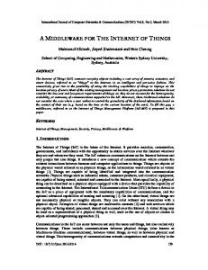
can be flat (row-like with a single level of data) or complex (tree-like/hierachical with multiple nested levels of data). We collected about 20,000 unique device schema from a one month period in January 2016 and analysed the structure of data. It was observed that out of 19,914 schema, 1542 (7.7%) are empty. From the non-empty schema, 18,280 (99.5%) are flat while 92 (0.5%) are complex. Hence, non-empty Dweet.io schema was almost always, flat (99.5%). The field count of a schema refers to the number of values in a flat schema besides the timestamp. Fig. 1 shows us the field counts of each flat device schema from Dweet.io. We found that 92.8% of the devices sampled had a schema of 2 or more fields attached on top of the timestamp. The majority (54.7%) had 4 fields attached to each timestamp. Hence, the schema indicates that sampled data on Dweet.io is largely wide. Our data is available on Github4 .

8+

Field Count

7 6 5 4 3 2 1 0

2000

4000

6000

8000

10000

Number of Schema

Fig. 1. Field counts from flat device schema

Therefore, through the study of public IoT device schema, we observe that our sample of over 20,000 unique IoT devices have data structures that are largely 1) flat and 2) wide (not just one, but multiple sensor values at a timestamp) . 2.1

Optimising for Time-Series IoT Data

We hypothesise that flat and wide data, made up of a timestamp and multiple sensor values, can be succinctly represented as rows and the necessary Linked Data produced ‘just-in-time’ for interoperability. As compared to representation as traditional Linked Data triples: 1. Storage is efficient as each field in a row stores just the value without additional subject and predicate values. 2. Queries that retrieve two or more fields from a row require no joins. 3. Metadata triples produced ‘just-in-time’ (e.g. the location of a sensor or unit of measure of its value) can be kept in-memory and need not be retrieved as data and joined. 4. Intermediate nodes (e.g. observation identifier connecting time instant and actual value) might seldom be used and can be abstracted from data 4

https://github.com/eugenesiow/iotdevices/releases/download/data/dweet_release.zip

4

Interoperable & Efficient: Linked Data for the Internet of Things

To realise this optimisation, we present our approach that involves mapping (a representation of abstracted metadata and data row bindings) and translation of queries from Linked Data SPARQL queries to row/relational SQL queries.

3

Mapping

Mapping serves the dual purpose of abstracting schema and metadata from actual sensor data stored as rows and providing bindings from that row data to Linked Data, allowing the translation of queries from SPARQL to SQL. We propose the SPARQL2SQL Mapping Language (S2SML), a simple and compact RDF-based language, designed with the structure of IoT data in mind, that is compatible with W3C recommendation, R2RML5 , for mapping. 3.1

Mapping as a Store of Abstracted Metadata

The difference and justification for S2SML over R2RML in the IoT is that S2SML mappings act like a Linked Data store for abstracted metadata (e.g. altitude of a sensor) and intermediate nodes (e.g. observation node connecting time instant, measurement data and sensor platform). It makes sense to abstract these to mappings as they are structurally different from the row data or are seldom projected from queries, however, they serve to connect and make Linked Data interoperable ‘just-in-time’. R2RML on the other hand is designed just for binding relational datasets to Linked Data. 3.2

Formal Definition of Mappings

Mappings and elements unique to S2SML are defined in Definitions 1, 2, 3, 4 and Table 1 gives descriptions and examples for each S2SML element. Definition 1 (S2SML Mappings, M ). Given a set of all possible S2SML mappings, M and a mapping, m ∈ M , a triple pattern, tp = (s, p, o) that is part of a mapping, tp ∈ m, has subject, s, predicate, p, and object, o where s = {I, Imap , B, F }, p = {I} and o = {I, Imap , B, L, Lmap , F }. Definition 2 (IRI Map, Imap ). An Imap is defined as a template that consists of the union of a set of IRI string parts, Ip and a set of table column binding strings, C, so Imap = Ip ∪ C and |C| >= 1, |Ip | >= 1. c is a string that consists of the table name and column separated by a 0 .0 character, enclosed within braces and c ∈ C. Definition 3 (Literal Map, Lmap ). An Lmap is defined as a RDF literal that consists of a table column binding string, c, as its value and a specific IRI, identifying it as an S2SML literal map as its datatype. c is a string that consists of the table name and column separated by a 0 .0 character. 5

http://www.w3.org/TR/r2rml/

Interoperable & Efficient: Linked Data for the Internet of Things

5

Definition 4 (Faux Node, F ). An F is defined as a template that consists of the union of a set of IRI string parts, Ip and a set of ID placeholders, Uid , so F = Ip ∪ Uid and |Uid | >= 1, |Ip | >= 1. u = {tablename.uuid} and u ∈ Uid .

Table 1. Examples of elements in (s, p, o) sets Symbol Name

Example

I Imap B L Lmap F

_:bNodeId "-111.88222"ˆˆ "readings.temperature"ˆˆ

3.3

IRI IRI Map Blank Node Literal Literal Map Faux Node

Mapping Closure

Devices and hubs might have multiple sets of row data and their corresponding mappings. We define a mapping closure in Definition 5 that allows us to represent this collection of multiple mappings on a device. Definition 5 (Mapping Closure, Mc ). Given the set of all mappings on a device, Md = {md |md ∈ M }, where M is a set of all possible S2SML S mappings. A mapping closure is the union of all elements in Md , so Mc = m∈Md m. 3.4

Implicit Join Conditions

Sensor data that is represented across multiple tables within a mapping closure might need to be joined if matched by a SPARQL query. In the R2RML specification, one or more join conditions (rr:joinCondition) may be specified between triple maps of different logical tables. In S2SML, these join conditions are automatically discovered as they are implicit within mapping closures from IRI template matching involving two or more tables. Definition 6 (IRI Template S Matching). S Following from Definition 2, Imap1 and Imap2 are matching if i1 ∈Ip i1 = i2 ∈Ip i2 and ∀i1 ∈ Ip1 , ∀i2 ∈ Ip2 : 1 2 pos(i1 ) = pos(i2 ) where pos(x) is a function that returns the position of x within its Imap . From matching IRI templates in the mapping closure, join conditions can be inferred. Given Definition 2 and 6, if c1 6= c2 , where c1 ∈ C1 , c2 ∈ C2 and pos(c1 ) = pos(c2 ), then, a join condition of c1 = c2 is required. Fig. 2 shows a mapping closure consisting of sensors and observations mappings. An IRI map, sen:system{sensors.name} and sen:system{readings.sensor}, in each of the mappings, fulfil a template matching. A join condition is inferred between the columns {sensors.name} and {readings.sensor} as a result.

6

Interoperable & Efficient: Linked Data for the Internet of Things

Fig. 2. Graph representation of an Implicit Join within a Mapping Closure

3.5

Cross Joins

Definition 7 (Table Selection, α). Given a SPARQL query q ∈ Q, where Q is a set of all possible SPARQL queries, and a mapping closure, Mc , a table selection function αMc (q) returns a set of table names required by the query and referenced by elements in the mapping closure. The output of α is used in the FROM clause of the translated SQL query. If there are tables in the FROM where there are no corresponding join conditions, a cross join, resulting in the cartesian product of two tables, is performed. This is possible in a mapping, m, within the mapping closure, Mc , that refers to two or more logical tables within its collection of Literal or IRI Maps.

3.6

Compatibility with R2RML

Although S2SML is more compact in terms of verbosity and can be processed by any existing SPARQL engines (without needing any additional structures, translation or algorithms) it can be translated to and from R2RML without losing expressiveness. Table 2 defines the other R2RML predicates and the corresponding S2SML construct. In particular, {rr:inverseExpression} is encoded within a literal, Liv , with a datatype of and the {rr:column} denoted with double braces {{COL2}}. is encoded by generating a named graph to group triples produced from that TripleMap and the query is stored in a literal object with context as the subject and as predicate as shown in Table 2.

Interoperable & Efficient: Linked Data for the Internet of Things

7

Table 2. Other R2RML predicates and the corresponding S2SML construct R2RML predicate

S2SML example

rr:language rr:datatype rr:inverseExpression rr:class rr:sqlQuery

"literal"@en "literal"ˆˆ "{COL1} = SUBSTRING({{COL2}}, 3)"ˆˆ ?s a . { ?p ?o.} s2s:sqlQuery "query".

Fig. 3. Translation Flow from SPARQL to SQL

4

Translation

The translation step is the process by which a Linked Data SPARQL query is applied to a mapping closure and translated to produce an SQL query that can be executed on the relational row store. Fig. 3 describes the process whereby: 1. A SPARQL Query is parsed to SPARQL Algebra with Jena ARQ6 . 2. Each Basic Graph Pattern (BGP) in the algebra is visited so that: – A mapping closure, Mc , is built from the set of mappings (Section 4.1). – The BGP is expressed as a SPARQL select query and executed using any SPARQL engine in-memory on the mapping closure (Section 4.2). – The result set is processed to produce a map of variable bindings (e.g. ?var, table1.col1), table selection (α, Definition 7) and join list (Section 3.4). 3. Other operators like FILTER, GROUP, UNION and PROJECT are visited and referencing the map of variable bindings, table selection α and join list, an SQL query is generated by doing syntax translation (Section 4.3). 6

https://jena.apache.org/documentation/query/

8

Interoperable & Efficient: Linked Data for the Internet of Things

4.1

Building a Mapping Closure

Following from Definition 5 of a Mapping Closure, Mc , a translation engine S needs to perform, m∈Md m, a union of all mappings on a device, Md . Giving consideration to template matching as described in Definition 6, we replace all Imap within each mapping m with Ip , the union of IRI string parts, and extract C, the set of table column binding strings. C is then stored as a global map, mjoin , with Ip as key and C as value. This map is used to produce the join list. In the example in Fig. 2, will replace and and mjoin will store under the key , the set {sensors.name, readings.sensor}. With this transformation, an Mc can be formed by adding all Md to it. This can be done using any triple store that can be queried with a SPARQL engine. 4.2

BGP Resolution with Swappable SPARQL engines

As mapping closures are standard Resource Description Format (RDF) triples, any SPARQL engine can perform BGP resolution. The BGP is expressed as a SPARQL select query (SELECT * WHERE {BGP}) and executed on a repository containing the mapping closure. We provide swappable Jena and OpenRDF Sesame engines in our implementation and a Java interface to extend to any other engine. Code is available on Github7 . 4.3

Operators and Syntax Translation

Definition 8 (Syntax Translation, trans). trans() is a function that takes a set of operators from SPARQL algebra, a table selection α, map of variable bindings, vmap , and join list, J, and returns syntax for an SQL query. The trans() function internally constructs an SQL query with clauses SELECT, FROM, WHERE, GROUP BY, HAVING, UNION, ORDER BY, LIMIT and OFFSET. BGP is just one of many operators that are visited from the SPARQL algebra and each operator when input into the trans function, either modifies one of the clauses or adds to the vmap , α and J. Table 3 shows a sample of clauses and the operators & maps that construct them. 4.4

Compression with Faux and Blank Nodes

Blank nodes, B and faux nodes, F help to compress intermediate nodes unlikely to be accessed by abstracting them to the mapping and only if they are retrieved from a BGP and PROJECT are they generated ‘just-in-time’. An ssn:Observation node in the SSN ontology can be connected to an ssn:SensorOutput, time:Instant and ssn:SensingDevice node. In turn an ssn:SensorOutput node is connected to a ssn:ObservationValue node which is connected to the actual value as a literal. The intermediate ssn:Observation, ssn:SensorOutput, 7

https://github.com/eugenesiow/sparql2sql

Interoperable & Efficient: Linked Data for the Internet of Things

9

Table 3. Example of operators and clauses bindings in translation Clause

Operators & Maps

SELECT FROM WHERE HAVING GROUP BY LIMIT

PROJECT, DISTINCT, UNION, vmap α J, FILTER, UNION FILTER GROUP, vmap SLICE

ssn:ObservationValue and time:Instant nodes are not required if we want to obtain the timestamp and the reading and can be compressed as B or F nodes. If the intermediate nodes are required for some reason, F nodes can be used. When F is input to a PROJECT operator, an SQL update statement, UPDATE table SET col=RANDOM_UUID(), is run to generate a row of identifiers and the Uid part of F in the mapping is updated from {table.uuid} to {table.col}.

5

Linked Data Infrastructure for IoT Scenarios

We note from Section 2 that IoT time-series sensor data from our sample is flat and wide. In this section, we focus on two specific IoT scenarios with flat and wide IoT data: a distributed meteorological analytics system of weather sensors and a personal smart home hub.

Fig. 4. Distributed Infrastructure for IoT Scenarios

In Fig. 4, we propose an inverse relationship between the level of distribution and compute and storage capability of components in a distributed architecture e.g. a cluster has high compute but cannot be distributed widely while sensors can be deployed widely but have minimal compute capability. Lightweight computers are compact and mobile machines that provide a balance of distribution and compute. We deploy our Linked Data Infrastructure on these lightweight computers, in close proximity to sensors and devices. The reference lightweight computer used is a Raspberry Pi 2 Model B+ with 1GB RAM, a 900MHz quadcore ARM Cortex-A7 CPU and a Class 10 SD Card.

10

Interoperable & Efficient: Linked Data for the Internet of Things

5.1

Distributed Meteorological System and SRBench

This IoT scenario uses the established Linked Sensor Data [9] dataset that describes sensor data from about 20,000 weather stations across the United States with recorded observations from periods of hurricanes and blizzards. We used the Nevada Blizzard, with about 100k triples for storage and performance tests and the largest 300k triple Hurricane Ike dataset in storage tests. At each station, there are a varying number of sensors (e.g. WindDirection, Rainfall) which produce observations at fixed intervals. This forms a stream of flat and wide rows of data. Each station and sensor also has metadata associated to it like the location, nearby stations or units of measure. Fig. 4 shows our design of the meteorological system. Lightweight computers serve as station hubs that store and make available for querying (as Linked Data) the stream of observations from weather sensors. An analytics hub on a server broadcasts queries to all station hubs and retrieves the results for visualisation. We performed a benchmark with SRBench [15], an analytics benchmark for Linked Sensor Data. The benchmark uses streaming SPARQL queries but can be applied, with similar effect, to SPARQL queries constrained by time. Queries 1 to 108 were used as they involve time-series sensor data while the remaining queries involved integration or federation with DBpedia or Geonames which was not within the scope of the experiment. Queries are available on Github9 . We transformed the Linked Sensor Data from Linked Data to row data10 . Due to resource constraints, we ran the benchmarks for each station in series on a Pi, which is similar to parallel execution on a network with low latency, recording individual times and taking the maximum time among all stations. 5.2

Smart Home Hub and Analytics Benchmark

In this scenario, we used data from smart home sensors collected by Barker et al. [2] over 3 months in 2012. We utilised a variety of data including environment sensors, motion sensors in each room and energy meter readings to devise a set of queries that require space-time aggregations for descriptive and diagnostic analytics. Queries can be found on this wiki11 and include 1) hourly aggregation of internal or external temperature 2) daily aggregation of temperature 3) hourly and room-based aggregation of energy usage 4) diagnose unattended energy usage with meter and motion, aggregating by hour and room. Fig. 4 shows our design of the smart home system with lightweight computers serving as the personal hub aggregating and storing sensor readings from energy meters, environment sensors, etc. Each device or sensor contributes a mapping in the mapping closure based on the SSN ontology12 . 8 9 10 11 12

http://www.w3.org/wiki/SRBench https://github.com/eugenesiow/sparql2sql/wiki https://github.com/eugenesiow/lsd-ETL https://github.com/eugenesiow/ldanalytics-PiSmartHome/wiki/ http://pi.webobservatory.me/info/datamodel

Interoperable & Efficient: Linked Data for the Internet of Things

5.3

11

Experiment

For both scenarios, we compared two Java-based database management systems, a traditional Linked Data store, TDB13 and our approach with S2SML mapping and S2S (SPARQL-to-SQL) translation on a row-based store, H214 . Both stores were run in disk-based mode. Ethernet connections were used between the client and the Pis’ to reduce network overhead for consistency. We took averages over 3 runs for each test. Running off the Java Virtual Machine on the Pis’ gave a consistent platform for benchmarking with 512mb the memory size allocated. We compared both storage efficiency and performance.

6

Results & Discussion

6.1

Storage Efficiency

Table 4 shows the difference in database storage sizes of different datasets for the S2S and TDB setups. As time-series sensor data benefits from the more succinct storage as rows, the S2S setup outperformed the Linked Data store, TDB, in terms of storage efficiency from one to two orders of magnitude. Furthermore, Linked Data stores rely on indexing all triples for performance [14] and TDB creates 3 triple indexes (OSP,POS,SPO) and 6 quad indexes to boost query performance. This increases storage size as observed. Table 4. Database Size By Dataset Dataset Nevada Blizzard Hurricane Ike Smart Home

6.2

S2S (mb) TDB (mb) %improve 90 761 135

6162 6847% 85274 11206% 2103 1558%

Query Performance

The performance of the two setups for the SRBench queries from the Nevada Blizzard are shown in Figure 5. Query performance for the S2S setup was from 3 times to 3 orders of magnitude better than the TDB setup. The S2S setup performs consistently well for all the queries with similar execution times whereas the TDB setup differs significantly on different queries. The S2S setup does not have to perform joins between tables for all queries and hence the stable average run times. The TDB setup performs much slower than the S2S setup on query 9 due to the join operation between two subtrees retrieved in the graph for two observations, WindSpeedObservation and WindDirectionObservation, being very time 13 14

https://jena.apache.org/documentation/tdb/ http://www.h2database.com/

Interoperable & Efficient: Linked Data for the Internet of Things Thousands

12

10

1328.20

47.08

9 8

Max Time Taken (ms)

7 6 5 4 3 2 1 0

1

2

3

4

5 Query

6

7

8

S2S

9

10 TDB

Fig. 5. SRBench Query Performance

Time Taken (ms) Thousands

consuming in the low-resource environment. An in-depth investigation showed the total query time was a 100 times more than the time to retrieve both subgraphs individually. Query 4 offers a similar situation with TemperatureObservation and WindSpeedObservation. The S2S setup, on the other hand, eliminates the need for this join as both observations belong to columns of the same row.

500

527

400 300 200 100 0

1

2

Query

3

S2S

4 TDB

Fig. 6. Smart Home Query Performance

Figure 6 shows the Smart Home query performance for the S2S and TDB setups. Again the S2S Setup performed better for all queries, from 3 to 70 times faster. Both S2S and TDB performed much faster on queries 1 and 2 than 3 and 4 as they involved disk access (a limiting factor due to the SD card) on a much smaller portion of the database - environment sensor readings as compared to motion and meter sensor readings. The S2S setup still produced an order of magnitude better performance due to reducing joins e.g. between timestamp and the internal temperature values recorded in the same row.

Interoperable & Efficient: Linked Data for the Internet of Things

13

Query 3 utilised smart meter data and query 4 involved both the smart meter and motion sensor data, a comparatively larger set of data and both did space and time aggregations on the data, hence, each took longer than the previous queries. Joins between tables (meter and motion) in Q4 affect both setups, as they belong to 2 different sensors, although the S2S setup still provides significant overall performance improvements in analytical queries. Table 5 summarises the results for both benchmarks. Table 5. Average Query Run Times of SRBench and Smart Home Scenarios SRBench TS2S (ms) TT DB (ms) %improve 1 2 3 4 5 6 7 8 9 10

6.3

365 415 375 533 415 457 455 320 436 354

1679 460% 1651 398% SmartHome TS2S (ms) TT DB (ms) %improve 1258 335% 47084 8839% 1 466 13709 2942% 1119 269% 2 2457 21898 891% 2751 602% 3 4685 322357 6881% 6563 1444% 4 147649 527184 357% 1785 558% 1328197 304865% 2514 709%

Overall Efficient Access

Our approach, represented by the S2S setup, improves both storage efficiency and query performance. Most queries can be answered in sub-second times which means efficient access to time-series sensor data by IoT applications is possible while maintaining interoperability through the use of Linked Data.

7

Impact on Privacy, Data Ownership & Data Locality

The use of lightweight computers as distributed hubs in our proposed infrastructure means that data that is collected from sensors and devices are stored and processed locally. As Vaquero et al. [13] state, data ownership will be a cornerstone of distributed IoT networks, where some applications will be able to use the network to run applications and manage data without relying on centralised services. This approach has an advantage over storing encrypted data in traditional clouds as a means to maintain privacy because it is easier to perform processing (no need for crypto-processors or applying special encryption functions) over such data. In our smart home scenario, the use of a personal hub on a lightweight computer based on an open ecosystem helps to mitigate the fears proposed by Albrecht et al. [1] that a mega corporation owns our data (and the local supermarket) and has little incentive to value our privacy. Roman et al. [12] further emphasise with their study of centralised and decentralised IoT infrastructures that when data is managed by the distributed entities, specific privacy

14

Interoperable & Efficient: Linked Data for the Internet of Things

policies and access control with additional trust and fault tolerance mechanisms can be created. Data locality is beneficial in the sense that we no longer need to send all the data around the world all the time. In disaster management IoT scenarios, where last-mile connectivity is lost, having data locality and offline access is especially valuable. An example is the Nepal earthquake in 2015 where last-mile connectivity was lost though global connectivity was maintained. Hence, our infrastructure that pushes both storage and compute to lightweight computers in edge networks within an open ecosystem, makes it more viable for end users to own their data. Specific privacy policies and technology can be built on top of this distributed infrastructure which has data locality as an added advantage. We show with our experiment that performance and storage efficiency for a variety of queries on data are sub-second and analytics-ready.

8

Related Work

SPARQL to SQL query translation has evolved with state-of-the-art engines like morph [10] and ontop [11] able to produce flatter & more efficient SQL queries. Both these engines, however, are designed for Ontology-Based Data Access (OBDA) or mapping relational stores to Linked Data with R2RML. Our work differs in that we build an R2RML-compatible mapping language that is additionally designed for the abstraction and storage of metadata within mappings. Secondly, we support the use of blank nodes (within the R2RML specification but not supported by other engines at the time of writing) and faux nodes to represent and compress intermediate nodes unlikely to be accessed. Lastly, we evaluate the performance of this approach on an IoT infrastructure with Pis’. Previous work on SPARQL to SQL translation by Chebotko et al. [6] helped to establish formally that the full separation of translation from the relational database schema design was possible and that efficient queries significantly improved query performance. While work by Elliot et al. has the same aims of efficient SQL queries but covers a smaller subset of SPARQL 1.0 e.g. no support date functions required for time aggregation in analytical queries.

9

Conclusion

Our approach of storing time-series data from IoT sensors in rows on lightweight computers and allowing Linked Data SPARQL queries through translation via mappings is shown to increase the performance of both storage and compute in two IoT scenarios as compared to traditional Linked Data stores. The improvement in storage and query performance is significant, 3 times to three orders of magnitude. More essentially, it allows most benchmark queries and space-time aggregations for analytics to run in sub-second, providing a basis for IoT applications working on sensor data. With Linked Data produced ‘just-in-time’, the approach supports interoperability without exchanging efficient access. The proposed infrastructure also shows how compute and storage in the IoT can be

Interoperable & Efficient: Linked Data for the Internet of Things

15

distributed to edge networks with lightweight computers which is a boon for privacy, data ownership and situations where last-mile access breaks down.

References 1. Albrecht, K., Michael, K.: Connected: To Everyone and Everything. IEEE Technology and Society Magazine pp. 31–34 (2013) 2. Barker, S., Mishra, A., Irwin, D., Cecchet, E.: Smart*: An open data set and tools for enabling research in sustainable homes. In: Proceedings of the Workshop on Data Mining Applications in Sustainability (2012) 3. Barnaghi, P., Wang, W.: Semantics for the Internet of Things: early progress and back to the future. International Journal on Semantic Web and Information Systems 8(1), 1–21 (2012) 4. Bizer, C., Heath, T., Berners-Lee, T.: Linked Data - The Story So Far. International Journal on Semantic Web and Information Systems 5, 1–22 (2009) 5. Buil-Aranda, C., Hogan, A.: SPARQL Web-Querying Infrastructure: Ready for Action? The Semantic Web - ISWC 2013 pp. 277–293 (2013) 6. Chebotko, A., Lu, S., Fotouhi, F.: Semantics preserving SPARQL-to-SQL translation. Data and Knowledge Engineering 68(10), 973–1000 (2009) 7. Heath, T., Bizer, C.: Linked Data Evolving the Web into a Global Data Space. In: Synthesis Lectures on the Semantic Web: Theory and Technology (2011) 8. International Telecommunication Union: Overview of the Internet of things. Tech. rep. (2012) 9. Patni, H., Henson, C., Sheth, A.: Linked Sensor Data. In: Proceedings of the International Symposium on Collaborative Technologies and Systems. pp. 362–370 (2010) 10. Priyatna, F., Corcho, O., Sequeda, J.: Formalisation and Experiences of R2RMLbased SPARQL to SQL Query Translation using Morph. Proceedings of the 23rd International Conference on World Wide Web pp. 479–489 (2014) 11. Rodriguez-Muro, M., Rezk, M.: Efficient SPARQL-to-SQL with R2RML mappings. Web Semantics: Science, Services and Agents on the World Wide Web 33, 141–169 (2014) 12. Roman, R., Zhou, J., Lopez, J.: On the features and challenges of security and privacy in distributed internet of things. Computer Networks 57(10), 2266–2279 (2013) 13. Vaquero, L.M., Rodero-Merino, L.: Finding your Way in the Fog: Towards a Comprehensive Definition of Fog Computing. ACM SIGCOMM Computer Communication Review 44(5), 27–32 (2014) 14. Weiss, C., Karras, P., Bernstein, A.: Hexastore: sextuple indexing for semantic web data management. Proceedings of the VLDB Endowment 1(1), 1008–1019 (2008) 15. Zhang, Y., Duc, P., Corcho, O., Calbimonte, J.P.: SRBench: A Streaming RDF/SPARQL Benchmark. The Semantic Web - ISWC 2012 7649, 641–657 (2012)