Apr 7, 2016 - opportunity (i.e., recommendation), he or she relies on eval- uating the rationale of ... recommendation performance, but also enables the discov- ery of interesting and ...... For BPR we used the python/theano implementation.
1
Interpretable recommendations via overlapping co-clusters
arXiv:1604.02071v1 [cs.IR] 7 Apr 2016
Reinhard Heckel and Michail Vlachos Abstract—There is an increasing need to provide not only accurate but also interpretable recommendations, in order to enhance transparency and trust in the recommendation process. This is particularly important in a business-to-business setting, where recommendations are generated for experienced sales staff and not directly for the end-client. In this paper, we consider the problem of generating interpretable recommendations based on the purchase history of clients, or more general, based on positive or one-class ratings only. We present an algorithm that generates recommendations by identifying overlapping co-clusters consisting of clients and products. Our algorithm uses matrix factorization techniques to identify co-clusters, and recommends a client-product pair because of its membership in one or more client-product co-clusters. The algorithm exhibits linear complexity in the number of co-clusters and input examples, and can therefore be applied to very large datasets. We show, both on a real client-product dataset from our institution, as well as on publicly available datasets, that the recommendation accuracy of our algorithm is better than or equivalent to standard interpretable and non-interpretable recommendation techniques, such as standard one-class nearest neighbor and matrix factorization techniques. Most importantly, our approach is capable of offering textually and visually interpretable recommendations.
F
1
I NTRODUCTION
In this paper, we consider the problem of providing interpretable client-product recommendations based on the purchase history of clients. The particular application we are interested in is a business-to-business (B2B) recommender system, in which the recipient of the recommendation is a sales person responsible for the client, and not the client itself. A salesperson is typically responsible for tens or hundreds of clients and to decide whether to pursue a sales opportunity (i.e., recommendation), he or she relies on evaluating the rationale of the recommendation. It is therefore particularly important to produce recommendations based on interpretable models, rather than on models that merely highlight the propensity of interest. Interpretability in general adds trust, confidence [11] and persuasiveness [47] to the recommendation, and in certain scenarios helps highlight tradeoffs and compromises [24] and even incorporates aspects of social endorsement [41]. Therefore, interpretable recommendations are of interest in many application areas. We base our recommendations on positive ratings only. In a business recommender system, positive ratings correspond to the purchase history of the clients, that is, the sets of products the clients have purchased. In this scenario, negative ratings are typically not available, as not purchasing a product does not reflect a negative rating. The problem of generating recommendations based on positive ratings of users only is known as One-Class Collaborative Filtering (OCCF). The lack of negative feedback makes this problem challenging, as one has to learn the customer preferences from what they like, without getting to see what the customers dislike. This problem also occurs in other important collaborative filtering settings, in particular when only implicit ratings are available. For example, a provider •
R. Heckel and M. Vlachos are with the Cognitive Systems group at IBM Research - Zurich.
of a news website faces the problem of generating article recommendations based on the readers’ historical article views. In such a setup, the readers do not provide explicit negative feedback. Equivalent OCCF tasks can be formulated from the browsing history of a visitor at an e-commerce website or when viewing videos on a video-sharing platform. Our approach to providing interpretable recommendations from positive examples is based on the detection of coclusters of clients that buy sets or bundles of products. The intuition behind this approach is that there exist clusters, groups, or communities of users that are interested in a subset of the items1 . These groups are called co-clusters because they consist of both users and items with similar patterns. Users can have several interests, and items might satisfy several needs, so users and items may belong to several co-clusters. This means that co-clusters may be overlapping. Our motivation for driving recommendations based on finding overlapping user-item co-clusters is that such an approach offers an interpretable model: Identification of sets of users that are interested in or have bought a set of items not only allows us to infer latent underlying patterns but can also lead to better, textually and visually interpretable recommendations. Standard state-of-the-art recommendation approaches based on matrix factorization are in general not applicable here, because of a lack of interpretability, as “latent factors obtained with mathematical methods applied to the useritem matrix can be hardly interpreted by humans” [32]. This observation has been made in several works [2], [33], [48]. Co-clustering principles have been considered before in the context of recommender systems [40], [18], but past work considered non-overlapping co-clusters only, where every item/user belongs to only one co-cluster. In fact, in the traditional co-clustering setting, co-clusters are also non1. In what follows, we use ‘item’ for ‘product’ and ‘user’ for ‘client’/‘company’, to conform with the standard literature on recommender systems
2
users
items
Fig. 1. Example of overlapping user-item co-clusters identified by the OCuLaR algorithm. Black rectangles correspond to positive examples, and the white squares within the clusters correspond to recommendations of the OCuLaR algorithm.
overlapping [8]. In contrast, in this work we use overlapping co-clusters to generate interpretable recommendations. Allowing co-clusters to overlap is not only crucial for the recommendation performance, but also enables the discovery of interesting and useful buying patterns. In Figure 1, we provide an example of overlapping co-clusters. A black dot describes a product bought by the user in the past. One can visually identify three potential recommendations indicated by white squares inside the co-clusters. The approach we propose identifies overlapping user-item co-clusters and generates recommendations based on a generative model. The algorithm is scalable, on par in terms of recommendation accuracy with state-of-art OCCF methodologies, and at the same time provides interpretable recommendations. Outline: The paper is organized as follows. We review related work in Section 2, and present our Overlapping coCLuster Recommendation algorithm, henceforth referred to as “OCuLaR”, in Section 4. We will first introduce a generative model, based on which we design a computationally efficient algorithm to produce recommendations and to identify the co-clusters. In Section 4.5, we explain the relation of traditional matrix factorization approaches to our algorithm, and in Section 6 we discuss how to add extra information into OCuLaR. Section 7 compares OCuLaR to other state-ofthe-art recommendation algorithms on a real-world clientproduct dataset from our institution and publicly available datasets. We show that our algorithm performs as well as or better than state-of-the-art matrix factorization techniques, with the added benefit of interpretability. Finally, in Section 8, we present and discuss a deployment of our algorithm in a B2B recommender system at our institution.
2
R ELATED W ORK
Collaborative Filtering (CF): Early approaches to recommender systems performed either user-based or item-based collaborative filtering. User-based techniques infer preferences of a given user based on the preferences of similar or like-minded users by, e.g., recommending products that the nearest neighbors of a user have bought in the past. Similarly, item-based techniques exploit item-to-item similarities to generate recommendations. Item- and userbased techniques yield a reasoning of the sort “similar users
have also bought”, but are often outperformed by latent factor models, such as matrix factorization approaches [19]. Matrix factorization techniques in their traditional form predict ratings or preferences well, but the latent features make it difficult to explain a recommendation [2], [33], [32]. Recently, [48] investigates a method for explainable factorization by extracting explicit factors (sentiment, keywords, etc) from user reviews; such an approach is applicable only in the presence of additional textual information for each recommendation. Such data, however, are rarely available in a B2B setting. Generic methodologies for communicating explanations to the user have been studied in [38], [11], [12]. Conceptually, the algorithm proposed in this work can be regarded as a combination of item-based and user-based approaches. Specifically, we discover similarities that span across both the user and the item space by identifying useritem co-clusters. By identifying user-item co-clusters via matrix factorization techniques, we obtain an estimate of the probability that an unknown example is positive, which automatically results in ranked recommendations. OCCF models are used to predict preferences from implicit feedback. This is a typical recommendation scenario when browsing, buying, or viewing history is available, or in general in setups where the user does not provide any explicit negative feedback. Recommendation techniques based on positive ratings try to learn by considering the implicit feedback either as absolute preferences [27], [16], or as relative preferences [31], [28]. We compare with techniques from both categories in Section 7, and state the formal relation of our approach to matrix factorization techniques in Section 4.5. Co-clustering: The majority of the literature on co-clustering considers the detection of non-overlapping co-clusters [10], [29]. Notable exceptions are the approach in [3], which introduces a generative model for overlapping co-clusters along with a generic alternating minimization algorithm for fitting the corresponding model to given data, and the approach in [36], which considers the problem of simultaneously clustering documents and terms. That latter approach is based on a generative model and estimation of the corresponding model parameters [36]. In both [3], [36], the focus is on discovering co-clusters, whereas here we are interested in explaining the recommendations produced by our algorithm with co-clusters. Although co-clustering approaches were used before in the collaborative filtering setting, the majority of those papers [13], [18], [40] is restricted to non-overlapping co-clusters. An exception is [44], which explores the multiclass co-clustering problem in the context of CF. Community detection: Related to co-clustering is community detection. To see this, observe that the positive examples are the edges in a bipartite graph of users and items (see Figure 1). Then, the co-clusters of users and items correspond to user-item communities in the bipartite graph. With the advent of social networking tools, interest in detecting communities of users that share the same interests has increased. Traditionally, community detection was formulated as a graph-partitioning problem (e.g., mincut); therefore the corresponding approaches in general do not tackle the case of overlapping communities. One of the
3
best-known community detection algorithms is based on the notion of modularity [25]. Specifically, the modularity algorithm by Girvan & Newman [14] is one of the most widely-used community detection algorithms and is used in many software packages (gephy, Mathematica, etc). It has the advantage that it can automatically discover the number of communities; however it does not support discovery of overlapping communities. Other work on detecting nonoverlapping communities includes [17], [9]. Recently, interest in identification of overlapping communities has grown [26], [1], [21], [45], [30]. Related to our work is the BIGCLAM algorithm proposed by Yang and Leskovec [45]; main differences are that in our approach we consider a particular bi-partite graph and use regularization, which turns out to be crucial for recommendation performance. In general, off-the-shelf community detection methodologies are not directly applicable to the one class collaborative filtering problem, as they yield an assignment of users/items to communities, but not a ranked list of recommendations.
3
by the K -dimensional co-cluster affiliation vectors fu and fi , respectively. The entries of fu , fi are constrained to be non-negative, and [fu ]c = 0 signifies that user u does not belong to co-cluster c. Here, [f ]c denotes the c-th entry of f . The absolute value of [fu ]c corresponds to the affiliation strength of u with co-cluster c; the larger it is, the stronger the affiliation. Positive examples are explained by the co-clusters as follows. If user u and item i both lie in co-cluster c, then this co-cluster generates a positive example with probability
1 − e−[fu ]c [fi ]c . Assuming that each co-cluster c = 1, ..., K , generates a positive example independently, it follows that Y 1 − P [rui = 1] = e−[fu ]c [fi ]c = e−hfu ,fi i , c
where hf , gi = Thus
OC U L A R ALGORITHM
In this section, we present our Overlapping co-CLuster Recommendation algorithm, or for short “OCuLaR”. We assume an underlying model whose parameters are factors associated with the users and items. Those factors are learned, such that the fitted model explains well the given positive examples rui = 1. The specific choice of our model has several advantages, e.g., it allows us to design an efficient algorithm to learn the factors. Moreover, the factors encode co-cluster membership and affiliation strength, and are interpretable in that sense. 4.1
(1)
P [rui = 1] = 1 − e−hfu ,fi i−bu −bi −b , we found that fitting the corresponding model does not increase the recommendation performance for the datasets considered in Section 7, and therefore will not discuss it further. Fitting the model parameters
Given a matrix R, we fit the model parameters by finding the most likely factors fu , fi to the matrix R by maximizing the likelihood (recall that we assume positive examples to be generated independently across co-clusters and across items and users in co-clusters): Y Y L= (1 − e−hfu ,fi i ) e−hfu ,fi i . (u,i) : rui =1
(u,i) : rui =0
Maximizing the likelihood is equivalent to minimizing the negative log-likelihood: X X − log L = − log(1 − e−hfu ,fi i ) + hfu , fi i . (u,i) : rui =1
Generative model
We start with the generative model underlying our recommendation approach. The generative model is similar to the BIGCLAM model [45] used for community detection. It formalizes the following intuition: There exist clusters, groups, or communities of users that are interested in a subset of the items. As users can have several interests, and items might satisfy several needs, each user and item can belong to several co-clusters consisting of users and items. However, a co-cluster must contain at least one user and one item, and can therefore not consist of users or items alone. Suppose there are K co-clusters (K can be determined from the data, e.g., by cross-validation, as discussed later). Affiliation of a user u and item i with a co-cluster is modeled
denotes the inner product in RK .
Note that so far the model cannot explain a positive example by means other than co-cluster affiliation. Although we could incorporate user, item, and overall bias by supposing that the probability of an example being positive is given by
4.2
4
c [f ]c [g]c
P [rui = 1] = 1 − e−hfu ,fi i .
F ORMAL PROBLEM STATEMENT
We are given a matrix R where the rows correspond e.g., to users or clients and the columns to items or products. If the (u, i)th element of R takes on the value rui = 1 this indicates that user u has purchased item i in the past or, more generally, that user u is interested in item i. We assume that all values rui that are not positive (rui = 1) are unknown (rui = 0) in the sense that user u might be interested in i or not. Our goal is to identify those items a user u is likely to be interested in. Put differently, we want to find the positives among the unknowns, given only positive examples.
P
(u,i) : rui =0
(2) To prevent overfitting, we add an `2 penalty, which results in the following optimization problem: minimize Q subject to [fu ]c , [fi ]c ≥ 0, for all c,
(3)
where
Q = − log L + λ
X i
2
kfi k2 + λ
X
2
kfu k2
(4)
u
and λ ≥ 0 is a regularization parameter. As will we discuss in more detail in Section 4.5, this optimization problem can be viewed as a variant of non-negative matrix factorization (NMF), specifically NMF with a certain cost function.
4
Choice of K : Recall that the number of co-clusters K is a model parameter. K can be determined from the data via cross-validation. Specifically, to determine a suitable K , we train a model on a subset of the given data for different choices of K , and select the K for which the corresponding model performs best on the test set. The model can thereby be tuned for an appropriate metric. In our experiments, we measure the recommendation performance in terms of the recall-at-M items [23], which is a standard performance metric in recommender system settings. 4.3
Generating interpretable recommendations
Suppose we want to recommend M items to each user. After having fitted the model parameters, we recommend item i to user u if rui is among the M largest values P [rui0 = 1], where i0 is over all items that user u did not purchase, i.e., over all i0 with rui0 = 0. The probability P [rui = 1] is large if the user-item pair (u, i) is in one or more user-item co-clusters. Thus, along with a recommendation, we can output the corresponding user-item co-clusters that cause P P [rui0 = 1] or, equivalently, hfu , fi i = [f ] [f u c i ]c to be c large. The user-item co-cluster c is determined as the subset of users and items for which [fu ]c and [fi ]c , respectively, are large.
items% 0% 1% 2% 3% 4% 5% 6% 7% 8% 9% 10% 11%
users%
A common approach to solve an NMF problem is alternating least squares, which iterates between fixing fu , and minimizing with respect to fi , and fixing fi and minimizing with respect to fu , until convergence. This strategy is known as cyclic block coordinate descent or the nonlinear Gauss-Seidel method. Whereas Q is non-convex in fi , fu , Q is convex in fi (with fu fixed) and convex in fu (with fi fixed). Therefore, a solution to the subproblems of minimizing Q with fixed fi and minimizing Q with fixed fu can be found, e.g., via gradient descent or Newton’s method. As this optimization problem is non-convex, one cannot in general guarantee convergence to a global minimum; however convergence to a stationary point can be ensured. Specifically, provided that λ > 0, Q is strongly convex in fi (with fu fixed) and in fu (with fi fixed). Thus, the subproblems have unique solutions, and therefore, if we solve each subproblem exactly, convergence to a stationary point is ensured by [4, Prop. 2.7.1]. However, as noted in the context of matrix factorization [15], solving the subproblems exactly may slow down convergence. Specifically, when fu , fi are far from a stationary point, it is intuitive that there is little reason to allocate computational resources to solve the subproblems exactly. It is therefore often more efficient to solve the subproblem only approximately in each iteration [5], [15]. For the above reasons, we will only approximately solve each subproblem by using a single step of projected gradient descent with backtracking line search, and iteratively update fi and fu by single projected gradient descent steps until convergence. In Section 4.4, we provide further implementation details. Convergence is declared if Q stops decreasing. This results in a very efficient algorithm that is essentially linear in the number of positive examples {(u, i) : rui = 1}, and the number of co-clusters K . Our simulations have shown that performing only one gradient descent step significantly speeds up the algorithm.
0% 1% 2% 3% 4% 5% 6% 7% 8% 9% 10% 11%
0%
0%
0%
.9%
.89%
.9%
.7%
0%
0%
0%
0%
0%
0%
0%
0%
.77%
.77%
.77%
.54%
0%
0%
0%
0%
0%
0%
0%
0%
.9%
.89%
.9%
.7%
0%
0%
0%
0%
0%
0%
0%
0%
0%
0%
0%
0%
0%
0%
0%
0%
0%
0%
.9%
.9%
.9%
.7%
0%
0%
0%
0%
0%
0%
0%
0%
.9%
.9%
.9%
.7%
0%
0%
0%
0%
0%
0%
0%
0%
.77%
.77%
.77%
.83%
.83%
.83%
.83%
.83%
.83%
0%
0%
0%
0%
0%
0%
.76%
.92%
.92%
.92%
.92%
.92%
0%
0%
0%
0%
0%
0%
.76%
.92%
.92%
.92%
.92%
.92%
0%
0%
0%
0%
0%
0%
.76%
.92%
.92%
.92%
.92%
.92%
0%
0%
0%
0%
0%
0%
0%
0%
0%
0%
0%
0%
0%
0%
0%
0%
0%
0%
0%
0%
0%
0%
0%
0%
0%
0%
“Item 4 is recommended to user 6 with confidence 83, because:
A. users 4 & 5 have purchased items 1-4 and us 6 has items 1-3.
B. Users 7,8,9 have purchase patterns of items 4-9, and user 6 has purchas item 5-9”
Fig. 2. The probability estimates P [rui ] = 1 − e−hfu ,fi i of the OCuLaR algorithm applied to the example in Figure 1; gray rectangles correspond to positive examples (rui = 1), white rectangles to unknown examples (rui = 0).
In the B2B setting that we consider it is also important to explicitly mention who are the clients that have purchased a similar bundle of products. Contrary to the B2C setting, where, for privacy reasons, one only mentions what similar clients purchase, in a B2B setting this is not a concern. The salesperson, who is the recipient of the recommendation, can use this information (explicit names of similar clients) to understand better the types of clients/companies that typically require such a solution. Our approach directly provides this information, because each co-cluster consists of specific clients (users) and products, and does not merely describe an average behavior. Example: Here we provide a cogent example about the interpretability of the recommendations by OCuLaR. We will use the user-item array from Figure 1. Let us consider making one recommendation to User 6, where Users 0–11 correspond to the rows, and Items 0–11 to the columns of the matrix. The probabilities of the fitted model for each useritem pair are depicted in Figure 2. The probability estimate P [rui ] = 1 − e−hfu ,fi i , for u = 6 is maximized among the unknown examples (rui = 0) for Item i = 4, and is given by 0.83. Therefore, OCuLaR recommends Item i = 4 to User u = 6. The corresponding factors are fi = [1.39, 0.73, 0.82] and fu = [0, 1.05, 1.25], which means that Item i = 4 is in all three co-clusters, while User u = 6 is in co-clusters 2 and 3 only. The probability estimate 1 − e−hfu ,fi i for u = 6, i = 4 is large because both User 6 and Item 4 are in co-clusters 2 and 3. To justify recommending Item 4 to User 6, we can therefore give the following, automatic interpretation to the user of the recommender system: Item 4 is recommended to Client 6 with confidence 0.83 because: •
•
Client 6 has purchased Items 1-3. Clients with similar purchase history (e.g., Clients 4-5) also bought Item 4. Moreover, Client 6 has purchased Items 5-9. Clients with similar purchase history (e.g., Clients 7-9) also bought Item 4.
5
Naturally, once the co-clusters have been discovered, additional information (derived from the co-clusters) can be attached in the rationale presented. In Section 6, we also discuss how additional information can be incorporated directly into the OCuLaR model. Finally, in the experimental Section 7, we discuss the recommendation rationale for an industrial deployment of OCuLaR (see Figure 6). 4.4
Implementation and complexity
Here we examine in more detail the projected gradient descent approach we use to solve the subproblems and the complexity of the overall optimization algorithm. It is sufficient to discuss minimization of Q with respect to fi , as minimization with respect to fu is equivalent. The following approach for minimizing Q was also used in similar form in [45], [22]. We start by noting that, because of ! X X X −hfu ,fi i Q= − log(1 − e )+ hfu , fi i
4.5
Relation to Matrix Factorization
Latent factor models are a prevalent approach to recommender systems. Among them, matrix factorization approaches are particularly popular, because of their good performance properties. In this section, we discuss the connection of our approach to standard matrix factorization techniques. Matrix factorization models in their most basic form represent users and items by latent vectors fu , fi in a low-dimensional space RK , and form a rating according to
rui = hfu , fi i . A common approach to fit the latent factors based on a given set of examples {rui } is to X 2 2 (7) minimize `(rui , hfi , fu i) + λkfi k2 + λkfu k2 , u,i 2
2
where ` is a loss function and kfi k2 , kfu k2 are regularization u : rui =1 u : rui =0 i terms to prevent overfitting. A common choice for nonX X 2 2 binary ratings is the quadratic loss function `(rui , hfi , fu i) = +λ kfu k2 + λ kfi k2 , (rui − hfi , fu i)2 . For the one-class collaborative filtering u i we can minimize Q for each fi individually. The part of Q problem, quadratic loss is not directly applicable, as the question remains on how to deal with the unknowns, for depending on fi is given by + * which rui = 0. Performing summation in (7) only over the X X 2 positive examples (rui = 1) is not sensible, as it results in a −hfu ,fi i fu +λkfi k2 . log(1 − e )+ fi , Q(fi ) = − trivial solution of fu = fi , for all u and all i to (7). A different u : rui =0 u : rui =1 (5) approach is to treat the unknowns as negative ratings. However, this might bias recommendations as some of the As mentioned, we update the parameter fi by performing unknown examples are actually positive ratings. To resolve a projected gradient descent step. The projected gradient this issue, it has been proposed in [27] to give different descent algorithm [4, Sec. 2.3] is initialized with a feasible weights to the error terms corresponding to positive and k+1 initial factor fi0 and updates the current solution fik to fi unknown ratings in the objective function, specifically to according to use the cost function ( fik+1 = (fik − αk ∇Q(fik ))+ , (rui − hfi , fu i)2 if rui = 1 `(rui , hfi , fu i) = , (8) where (f )+ projects f on its positive part, [(f )+ ]c = 2 b(rui − hfi , fu i) if rui = 0 max(0, [f ]c ), and the gradient is given by where b < 1 is a weight assigned to unknown ratings. A X X e−hfu ,fi i fu ∇Q(fi ) = − fu + 2λfi . + common approach to solve the corresponding optimization −hf ,f i 1−e u i u : rui =1 u : rui =0 problem is weighted alternating least squares (wALS) [27]. (6) Our approach is equivalent to choosing the loss function The step size αk is selected using a backtracking line search, `(rui , hfi , fu i) = − log(|rui − e−hfi ,fu i |). (9) also referred to as the Armijo rule along the projection arc [4]. Specifically, αk = β tk , where tk is the smallest positive integer such that D E Q(fik+1 ) − Q(fik ) ≤ σ ∇Q(fik ), fik+1 − fik where σ, β ∈ (0, 1) are user-set constants. PAs the computation of both ∇Q(fi ) and Q(fi ) requires u : rui =0 fu , and typically, the number of items for which rui = 1 is P small relative to the total number of items, we precompute u fu P before updating all fi , and then compute u : rui =0 fu via X X X fu = fu − fu . u : rui =0
u
P
u : rui =1
Using the precomputed u : rui =0 fu , a gradient descent step of updating fi has cost O(|{u : rui = 1}|K). Thus, updating all fi and all fu has cost O(|{(i, u) : rui = 1}|K), which means that updating all factors has a cost that is linear in the problem size (i.e., number of positive examples) and linear in the number of co-clusters.
This results in a large penalty if hfi , fu i is small for a positive example rui = 1, and a moderate penalty if hfi , fu i is large for an unknown example rui = 0. Our approach is therefore similar in spirit to that of giving different weights to positive (rui = 1) and unknown (rui = 0) examples. Interpretability: Matrix factorization approaches, such as the wALS algorithm (with loss function (8)), yield good empirical performance, as we will see in the experiments. Their main disadvantage for our scenario is that the latent space is typically not easy to interpret. This drawback of MF techniques is attested in various studies [20], [2], [33], [39]. This statement also applies to standard non-negative matrix factorization (NMF) techniques, where the factors are constraint to be non-negative. Our approach also uses factorization principles, however, we confine the factors to explicitly model user and item participation, which is key for not compromising the model interpretability.
6
5
R ELATIVE OC U L A R ALGORITHM (R-OC U L AR )
As we saw in the related work section, OCCF problems can be viewed as learning of either absolute or relative preferences of users. The OCuLaR algorithm belongs to the first category because it tries to learn the absolute ratings of the users. Specifically, as we saw, OCuLar can be viewed as a non-negative matrix factorization approach with a particular loss function (i.e., (9)), with the loss function assigning a large penalty to positive examples that are not well explained by the model (i.e., hfi , fu i small for rui = 1), and only a moderate penalty to unknown examples that are not well explained by the model (i.e., hfi , fu i large for rui = 0). In this section, we examine how OCuLaR could be adapted to treat the positive examples as relative preferences. The notion of relative preferences in OCCF was first explored by Rendle et al. [31], who proposed to predict the relative preferences (u prefers i over j ) rather than the absolute rankings. The underlying idea for this case is that there is an associated latent personalized ranking >u for each user u, where i >u j signifies that user u prefers item i over item j . To this end, in a first step, one can construct a “training” item ranking set for each user from the set of positive examples, denoted by S = {(u, i) : rui = 1}. The underlying assumption for this constuction is that, if rui = 1, then user u prefers item i item over all items j with unknown rating, i.e., ruj = 0. Specifically, the training item ranking data set DS is defined as:
DS = {(u, i, j) : rui = 1 and ruj = 0}. Note that negative examples are accounted for implicitly because if (u, i, j) ∈ DS , then j is not prefered over i. Triplets not in DS correspond to triplets for which no direct preference information is available; it is those triplets for which we want to learn the preferences. As shown in [31], assuming that the users act independently of each other and that >u is independent across u, the model likelihood can be maximized by maximizing Y P [i >u j] . (10) (u,i,j)∈DS
To adapt the notion of relative preferences for OCuLaR, suppose that the probability of a user preferring item i over item j is given by
P [i >u j] = (1 − e−hfu ,fi i )e−hfu ,fj i . To see the formal relation to the model in Section 4.1, simply note that, with this choice,
P [i >u j] = P [rui = 1] P [ruj = 0] with P [rui = 1] as defined in (1). Maximizing (10) is equivalent to minimizing the logarithm of (10), i.e., minimizing Y P [i >u j|θ] (u,i,j)∈DS
=
X
(log P [rui = 1] + log P [ruj = 0])
(u,i,j)∈DS
=
X
X
X
u i : rui =1 j : ruj =0
(log P [rui = 1] + log P [ruj = 0])
=
X
X
|{j : ruj = 0}|
u
log P [rui = 1]
i : rui =1
X
+ |{i : rui = 1}|
log P [ruj = 0]
j : ruj =0
∝
X
wu
u
=
X i : rui =1
X
X
log P [rui = 1] +
log P [ruj = 0]
j : ruj =0
X
wu log(1 − e−hfu ,fi i ) −
(u,i) : rui =1
hfu , fi i
(u,j) : ruj =0 |{i : r
=0}|
. Note that the RHS where we defined wu = |{i : rui ui =1}| above differs only in the factors wu from the negative loglikelihood (2) in Section 4.2. The factors wu assign a large weight to positive examples of users that have few positive examples associated with them. We denote the algorithm obtained by substituting the log-likelihood − log L in Section 4.2 with the RHS above as the relative OCuLaR (R-OCuLaR) algorithm. Its implementation is essentially equivalent to that of the (original) OCuLaR algorithm; in fact, it has exactly the same complexity.
6
A DDING EXTRA INFORMATION
While the focus of this paper is on generating recommendations based on positive examples only, e.g., on the purchase history of clients, we briefly explain the incorporation of additional information in the OCuLaR algorithm in this section. This is important for addressing the cold-start problem, i.e., for making recommendations to users that have no purchase history, or for recommending items that have not been purchased. In addition, it can also improve the recommendation performance for users/items for which positive examples exist. Additional information can be of the form of user and item attributes, such as the affiliation of a user or item with a certain hierarchy or ontology. For example, in the B2B setting, a client-company belongs to a certain industry (automotive, banking, etc.), and in the traditional consumer setting, a movie or a book belongs to one or more genres (biography, fiction, etc.). We restrict our attention to the incorporation of a single categorical item attribute, denoted by Ai , that takes on values in a finite set {a1 , ..., aJ }. The extension to several (distinct) item attributes and to user attributes will turn out to be straightforward. The item attribute is incorporated into the generative model by assuming that the attribute values Ai are generated by the co-cluster affiliations, similarly as the positive examples are generated by the co-cluster affiliations (cf. Section 4.1). This approach is quite common; for example, in the context of article recommendations, the collaborative topic model [42] assumes that article ratings are generated by latent vectors and by topic proportions (i.e., by item attributes). Similarly, binary features can be incorporated into the community model by proposing a model that generates both node attributes and edges in the corresponding graph with communities by regarding the community affiliation vectors as the inputs features to a (binary) logistic model [46]. In the same way, we assume that the Ai are generated by the co-clusters by regarding the co-cluster affiliation vectors
7
fu , fi as input features to a logistic model. Specifically, the probability of Ai taking on the value ak is given by
7.1
Datasets
We use four datasets. First, we consider a real-world dataset from our institution. It consists of the buying history of e−w0k −hwk ,fi i , k = 1, ..., J − 1, 80,000 clients with whom our institution interacts and 3,000 P [Ai = ak |F] = P −w0` −hw` ,fi i products or services offered by our institution. The clients e 1 + J−1 `=1 in this case are not individuals but companies, and the 1 P [Ai = aJ |F] = PJ−1 −w −hw ,f i , recommender system operates in an B2B setting. We call i 0` ` 1 + `=1 e this dataset B2B-DB. The dataset is highly imbalanced in the sense that the most frequently purchased item was where w0` , w` ∈ RK , ` = 1, ..., J − 1, are the associated bought by more than 50% of the users, whereas the most weight factors, and F contains fu , fi as columns. Assuming infrequently purchased item was bought only 50 times. that attributes are generated independently for each item, We also consider three public datasets. The first was the attribute likelihood is given by extracted by [43] from the CiteULike website, which assists Y users in creating collections of scientific articles. The dataset LA = P [Ai |F, W] , consists of 5,551 users and 16,980 articles. Each user has a i number of articles in their collection, which are considered where the product is over all items i that have a feature as positive examples. Based on the positive examples, the associated with them, and W denotes the set of associated goal is to generate new article recommendations. The secweight factors w0` , w` ∈ RK , ` = 1, ..., J − 1. Assuming ond dataset is the Movielens 1 million dataset, which consists that the positive examples and the attributes are generated of 1 million ratings from 6,000 users on 4,000 movies. The independently based on the community membership, the final dataset is the Netflix dataset, consisting of about 100 negative model log likelihood of the overall model is given millions ratings that 480,189 users gave to 17,770 movies. In both the Movielens and the Netflix dataset, the users by − log L˜ = − log L − µ log LA , where µ is a parameprovide ratings between 1 and 5 stars. As we consider a ter that weights the likelihoods. To find the factors fu , fi one-class collaborative filtering task, we adopt a convention and the weights of the logistic model w0` , w` , we solve— from many previous works (e.g., [28], [37]) and only conanalogously as in (3)—the following optimization problem: sider ratings larger than or equal to 3 as positive examples and ignore all other ratings. Therefore, the task now is ˜ subject to [fu ]c , [fi ]c ≥ 0, ∀c, minimize Q (11) equivalent to predicting whether the user will give a rating greater than 3 (i.e., is likely to enjoy the movie). where
˜ = − log L − µ log LA + λ Q
X i
2
kfi k2 + λ
X
2
kfu k2 .
u
Here, λ ≥ 0 is a regularization parameter, and minimization is with respect to the factors fu , fi and the weights w0` , w` . Similarly as before, one can use a cyclic block coordinate descent approach to minimize (11). Specifically, we iteratively update first fu , then fi , both via projected gradient descent, and finally the weights w0` , w` , with gradient descent. We finally note that this variant of OCuLaR is very efficient; specifically, the complexity of updating all factors and weights is O(|{(i, u) : rui = 1}|K + JKN ), where N is the number of items.
7
E XPERIMENTS
Here, we compare the prediction accuracy of OCuLaR to that of other interpretable and non-interpretable one-class CF algorithms. We compare with interpretable user-based and item-based collaborative filtering approaches, and noninterpretable state-of-art one-class recommendation algorithms based on matrix factorization. Both OCuLaR and R-OCuLaR typically outperform or are on par with the existing one-class recommendation algorithms in terms of recommendation performance. We also discuss the choice of the input parameters for our approach. We demonstrate that OCuLaR is scalable and easily parallelizable, and we conclude with an industrial deployment.
7.2
Recommendation performance
7.2.1 Evaluation Metrics We measure performance in terms of recall at M items (recall@M ), and mean average precision at M items (MAP@M). In the one-class setting, recall is a more sensible measure than precision, because an example being unknown (rui = 0) does not mean that user u would not rate item i positively [35]. Given an ordered (by relevance) list of M recommendations for user u, denoted by i1 , ..., iM , the recall@M items for user u is defined as |{i : rui = 1} ∩ {i1 , ..., iM }| recall@M (u) = . |{i : rui = 1}| The overall recall@M is obtained as the average over recall@M (u). MAP is commonly used in information retrieval for evaluating a ranked or ordered list of items, and is considered a good measure of performance when a short list of the most relevant items is shown to a user. MAP@M items is the mean (over all users) of the average precision at M items (AP@M), defined as M X 1{ruim =1} AP@M (u) = Prec(m) , min(|{i : rui = 1}|, M ) m=1 where |{i : rui = 1}| is the number of positive examples corresponding to user u; 1{ruim =1} is equal to 1 if ruim = 1 and zero otherwise, and Prec(m) is the precision at a cutoff rate m: |{i : rui = 1} ∩ {i1 , ..., im }| Prec(m) = . m
8
TABLE 1 Comparison of OCuLaR and R-OCuLaR with other baseline one-class recommendation algorithms.
dataset Movielens CiteULike B2B-DB
metric MAP@50 recall@50 MAP@50 recall@50 MAP@50 recall@50
OCuLaR
R-OCuLaR
.1809 .4021 .0906 .3042 .1801 .5240
.1805 .4086 .0916 .3177 .1651 .4780
Note that because Prec(m) ∈ [0, 1], we have that AP@M ≤ 1. 7.2.2 Comparison with baselines We compare the OCuLaR algorithm with various interpretable and non-interpretable baseline algorithms: •
•
•
•
User-based collaborative filtering using a cosine similarity metric [34]. Such an algorithm is interpretable because a recommendation can be justified with a reasoning of the type: “item i is recommended because the similar users u1 , .., uk also bought item i”. Item-based collaborative filtering using cosine similarity [7]. This algorithm is also interpretable. It can be accompanied with a recommendation such as: “item i is recommended because user u bought the similar items i1 , ..., ik ”. Weighted Alternating Least Squares (wALS), a stateof- the-art one-class matrix factorization approach [27]. wALS minimizes (7) with loss function (8) by alternatingly optimizing the user and the item factor via least-squares. It offers good prediction performance but the reasoning is not directly interpretable, as mentioned earlier. Bayesian personalized ranking (BPR), a state-of-theart matrix factorization approach that converts the set of positive examples into a set of relative preferences [31] (see also Section 5). The recommendations provided by BPR are also not directly interpretable. For BPR we used the python/theano implementation from https://github.com/bbcrd/theano-bpr.git.
All approaches require the setting of hyperparameters. To make the comparison fair, we try to find the best set of hyperparameters using a grid search approach. We do not consider the variant of OCuLaR which uses extra information for fairness to the baseline techniques that use only the matrix of positive examples. For OCuLaR and R-OCuLaR, we performed a grid search over K and λ. For the user- and item-based collaborative filtering approaches, we performed a grid search over the number of nearest neighbors. For wALS, we choose the weight in the loss function (8) as b = 0.01, the regularization parameter as λ = 0.01, and performed a grid search over the dimension of the latent vectors. Finally, for BPR we searched over the dimension of the latent factors K , and the regularization parameter λ. In Table 1, we plot the results obtained with the parameters that yield the best recall@50 for each approach2 . The recall@M and MAP@M values were obtained by splitting 2. Netflix dataset is not included because not all baselines can be run for very large datasets
wALS [27], [16] .1513 .3982 .1003 .3331 .1749 .5283
BPR [31] .1434 .3587 .0157 .0801 .1325 .4407
userbased [34] .1639 .3757 .0882 .2699 .1797 .4995
itembased [7] .1329 .3238 .1287 .2921 .1568 .4840
the datasets into a training and a test dataset, with a splitting ratio of training/test of 75/25, and averaging over 10 problem instances. We also plot the same results for recall@M and MAP@M for the Movielens dataset for varying M in Figure 3. The results across all datasets show that OCuLaR and R-OCuLaR are either the best or the second-best performing algorithm (together with wALS). In addition, OCuLaR has the advantage of providing interpretable recommendations, an aspect that is compromised when using other OCCF approaches such as wALS or BPR. Moreover, OCuLaR is significantly better than the user- and item-based algorithms, its interpretable competitors. This is not surprising because the user- and item-based approaches both consider only clustering in either the user or the item space, whereas OCuLaR can discover more complex structures in the joint user-item space. recall@M items
0.6
MAP@M items
R-OCuLaR OCuLaR
OCuLaR R-OCuLaR
0.2 0.4 R-OCuLaR
0.1
OCuLaR
0.2
wALS User-based BPR
0
0 0
50
100 M
Item-based
0
50
100 M
Fig. 3. Comparison of OCuLaR with baseline algorithms for the Movielens dataset.
7.3
OCuLaR parameters
We briefly discuss how to set the parameters for OCuLaR, as well the impact of this choice. Recall that OCuLaR expects the number of co-clusters K and the regularization parameter λ. Typically, values for K and λ are chosen such that the recommendation performance is optimized for a particular metric, as determined via cross-validation. In Figure 4, we show on the MovieLens dataset the impact of the parameter values on the recommendation performance and on a number of co-cluster properties. The top panel shows the recall@50 items. The graph demonstrates that too little (λ = 0) or too much regularization (λ = 100) can hurt the recommendation accuracy. K may be selected in such a way to ensure that the size of the
co-clusters is neither too big nor too small, and also that each user or item does not belong to too many co-clusters.The size of the co-clusters can depend on application-specific criteria, such as, for example, that a co-cluster should contain at least 100 users. For the specific example, a value of K in the range between 100-200 would be adequate to ensure good prediction and avoid excessively big, thus not dense, co-clusters. λ = 0
λ = 30
λ = 100
0.2 0.18 recall@50 items 0.16 0.14 users in co-cluster items in co-cluster
running time (sec/it)
9
300
K = 10
200
K = 50
200
K = 100
150
100
100 0 0
0.5
1
fraction of netflix dataset
0
5
10
number of threads
Fig. 5. Left: Running time per iteration of the OCuLaR algorithm applied to a fraction of the Netflix dataset. Right: Running time per iteration on the Netflix dataset as a function of the the number of threads.
1,000 500
to the clients of our institution, but rather to our sales teams. The salesperson responsible for an account examines the recommendations provided and decides whether to act on the recommendation and approach the client. This decision is based on the reasoning provided and on the salesperson’s own experience through past interaction with the client. The textual output of the recommendation, which conveys the corresponding rationale is shown in Figure 6. For reasons of anonymity, the names of the companies/clients belonging to each co-cluster have been omitted.
3,000 2,000 1,000
co-cluster densities
0.2 0.1
co-clusters an item is in
20 10
co-clusters a user is in
40 20 0
0
100
200
Fig. 4. Recall and various co-cluster metrics forKvarying values of the OCuLaR parameters K and λ.
7.4
Scalability
In this section, we investigate the scalability of the OCuLaR algorithm. We consider the full Netflix dataset, consisting of 100, 480, 507 ratings from 480, 189 users on 17, 770 movie titles. As before, we take the ratings ≥ 3 as positive examples, i.e., rui = 1. As analyzed in Section 4.4, the training time required by the OCuLaR algorithm is essentially linear in the number of positive examples |{(u, i) : rui = 1}|, and linear in the number of co-clusters K . In Figure 5 we plot the running time per iteration for increasing fractions of the Netflix dataset (i.e., non-zero entries), chosen uniformly from the whole Netflix dataset. We see that the training time is indeed linear in the number of positive examples |{(u, i) : rui = 1}| and linear in the number of co-clusters K. OCuLaR can also easily be parallelized because for an item (user) update cycle, each item (user) factor can be updated independently. Therefore independent threads can update a fraction of the user and item factors. Figure 5 depicts the reduction in running time that can be realized by the corresponding parallel OCuLaR implementation as a function of the number of threads.
8
I NDUSTRIAL DEPLOYMENT
We used our algorithm in a B2B recommender system of our institution. These recommendations are not offered directly
Fig. 6. Example from industrial deployment (client names are suppressed). Product “Custom Cloud” is recommended to Client 1 because the client is affiliated with three co-clusters. Co-cluster 1 shows an affinity of Client 1 with several airlines, and in Co-cluster 3 with telco companies.
In the example, it can be seen that the service “Custom Cloud” is recommended for “Client 1” with a confidence of 65.4%. The reasoning explains that Client 1 belongs to three co-clusters of other clients that have bought the same service as well as products similar to the ones that Client 1 has already purchased. Also, based on the co-clusters discovered the recommendation offered presents a price estimate of the potential business deal, based on historical purchases of the same product by the related clients belonging to the co-clusters discovered. During the deployment of the OCuLaR algorithm in our organization, we interacted with many sellers that used the platform. Sellers expressed satisfaction about the reasoned
10
aspect of the recommendations. An interesting comment that we received is that the tool could also constitute an educational platform [6] for young sellers, because the detailed reasoning can teach them the currently discovered buying patterns. In an extended version, we plan to provide additional metrics, such as the conversion ratio and the monetary benefits of the industrial deployment.
9
C ONCLUSION
A large amount of work on recommender systems and machine learning has focused primarily on the accuracy of prediction rather than on interpretability. This work explicitly addresses the aspect of interpretability by enabling the detection of overlapping co-clusters that can be easily visualized and transcribed into a textual description. The methodology presented is interpretable and at the same time scalable. More importantly, our approach does not sacrifice accuracy of prediction.
10
ACKNOWLEDGEMENTS
The research leading to these results has received funding from the European Research Council under the European Union’s Seventh Framework Programme (FP7/2007-2013) / ERC grant agreement no. 259569.
R EFERENCES [1] [2] [3] [4] [5] [6] [7] [8] [9] [10] [11] [12] [13] [14] [15] [16]
E. M. Airoldi, D. M. Blei, S. E. Fienberg, and E. P. Xing. Mixed membership stochastic blockmodels. In Advances in Neural Information Processing Systems, pages 33–40, 2009. M. Aleksandrova, A. Brun, A. Boyer, and O. Chertov. What about interpreting features in matrix factorization-based recommender systems as users? In Hypertext, 2014. A. Banerjee, C. Krumpelman, J. Ghosh, S. Basu, and R. J. Mooney. Model-based overlapping clustering. In Proc. ACM SIGKDD, pages 532–537, 2005. D. P. Bertsekas. Nonlinear Programming. Athena Scientific, 1999. S. Bonettini. Inexact block coordinate descent methods with application to non-negative matrix factorization. IMA J. Numer. Anal., 31(4):1431–1452, 2011. S. Cleger, J. Fernandez-Luna, and J. F. Huete. Learning from explanations in recommender systems. Inf. Sciences, 287:90–108, 2014. M. Deshpande and G. Karypis. Item-based top-N recommendation algorithms. ACM Trans. Inf. Syst., 22(1):143–177, 2004. I. S. Dhillon. Co-clustering documents and words using bipartite spectral graph partitioning. In Proc. ACM SIGKDD, pages 269–274, 2001. I. S. Dhillon, Y. Guan, and B. Kulis. Weighted graph cuts without eigenvectors–a multilevel approach. IEEE Trans. Pattern Analysis and Machine Intell., 29(11):1944–1957, 2007. I. S. Dhillon, S. Mallela, and D. S. Modha. Information-theoretic co-clustering. In Proc. ACM SIGKDD, pages 89–98, 2003. G. Friedrich and M. Zanker. A taxonomy for generating explanations in recommender systems. AI Magazine, 32(3):90–98, 2011. F. Gedikli, D. Jannach, and M. Ge. How should i explain? a comparison of different explanation types for recommender systems. J. Human-Computer Studies, 72(4):367–382, 2014. T. George and S. Merugu. A scalable collaborative filtering framework based on co-clustering. In Proc. ICDM, pages 625–628, 2005. M. Girvan and M. E. J. Newman. Community structure in social and biological networks. Proc. of the National Academy of Sciences, 99(12):7821–7826, 2002. C.-J. Hsieh and I. S. Dhillon. Fast coordinate descent methods with variable selection for non-negative matrix factorization. In Proc. ACM SIGKDD, pages 1064–1072, 2011. Y. Hu, Y. Koren, and C. Volinsky. Collaborative filtering for implicit feedback datasets. In Proc. ICDM, pages 263–272, 2008.
[17] G. Karypis and V. Kumar. Multilevel k-way partitioning scheme for irregular graphs. J. Parallel and Distributed Computing, 48(1):96– 129, 1998. [18] M. Khoshneshin and W. N. Street. Incremental collaborative filtering via evolutionary co-clustering. In Proc. RecSys, pages 325– 328, 2010. [19] Y. Koren, R. M. Bell, and C. Volinsky. Matrix factorization techniques for recommender systems. IEEE Computer, 42(8):30–37, 2009. [20] D. D. Lee and H. S. Seung. Learning the parts of objects by nonnegative matrix factorization. Nature, 401(6755):788–791, 1999. [21] J. Leskovec and J. J. Mcauley. Learning to discover social circles in ego networks. In Advances in Neural Information Processing Systems, pages 539–547, 2012. [22] C.-J. Lin. Projected gradient methods for nonnegative matrix factorization. Neural Computation, 19(10):2756–2779, 2007. [23] F. McSherry and M. Najork. Computing information retrieval performance measures efficiently in the presence of tied scores. In Proc. ECIR, pages 414–421, 2008. [24] K. Muhammad, A. Lawlor, R. Rafter, and B. Smyth. Great explanations: Opinionated explanations for recommendations. In Proc. ICCBR, pages 244–258, 2015. [25] M. E. J. Newman. Modularity and community structure in networks. Proc. of the National Academy of Sciences, 103(23):8577–8582, 2006. [26] G. Palla, I. Der´enyi, I. Farkas, and T. Vicsek. Uncovering the overlapping community structure of complex networks in nature and society. Nature, 435(7043):814–818, 2005. [27] R. Pan, Y. Zhou, B. Cao, N. Liu, R. Lukose, M. Scholz, and Q. Yang. One-class collaborative filtering. In Proc. ICDM, pages 502–511, 2008. [28] W. Pan and L. Chen. GBPR: group preference based bayesian personalized ranking for one-class collaborative filtering. In Proc. IJCAI, pages 2691–2697, 2013. [29] S. Papadimitriou and J. Sun. Disco: Distributed co-clustering with map-reduce: A case study towards petabyte-scale end-to-end mining. In Proc. ICDM, pages 512–521, 2008. [30] T. P. Peixoto. Model selection and hypothesis testing for large-scale network models with overlapping groups. CoRR, abs/1409.3059, 2014. [31] S. Rendle, C. Freudenthaler, Z. Gantner, and L. Schmidt-Thieme. BPR: bayesian personalized ranking from implicit feedback. In Proc. UAI, pages 452–461, 2009. [32] M. Rossetti, F. Stella, and M. Zanker. Towards explaining latent factors with topic models in collaborative recommender systems. In DEXA, Workshop, pages 162–167, 2013. [33] S. Roy, R. Homayouni, M. Berry, and A. Puretskiy. Nonnegative tensor factorization of biomedical literature for analysis of genomic data. In K. Yada, editor, Data Mining for Service, volume 3 of Studies in Big Data, pages 97–110. 2014. [34] B. M. Sarwar, G. Karypis, J. A. Konstan, and J. Riedl. Analysis of recommendation algorithms for e-commerce. In Proc. EC, pages 158–167, 2000. [35] A. I. Schein, A. Popescul, L. H. Ungar, and D. M. Pennock. Methods and metrics for cold-start recommendations. In Proc. ACM SIGIR, pages 253–260, 2002. [36] M. M. Shafiei and E. E. Milios. Latent Dirichlet co-clustering. In Proc. ICDM, pages 542–551, 2006. [37] V. Sindhwani, S. S. Bucak, J. Hu, and A. Mojsilovic. A family of non-negative matrix factorizations for one-class collaborative filtering problems. In RecSys Workshop, 2009. [38] N. Tintarev and J. Masthoff. A survey of explanations in recommender systems. In Proc. ICDEW, pages 801–810, 2007. [39] S. Venkatasubramanian. New developments in nonnegative matrix factorization. www.cs.utah.edu/∼suresh/papers/column/ nmf/nmf-mod.pdf, 2013. [Online; accessed Oct-15]. [40] M. Vlachos, F. Fusco, C. Mavroforakis, A. T. Kyrillidis, and V. G. Vassiliadis. Improving co-cluster quality with application to product recommendations. In Proc. CIKM, pages 679–688, 2014. [41] B. Wang, M. Ester, J. Bu, and D. Cai. Who also likes it? generating the most persuasive social explanations in recommender systems. In Proc. AAAI, pages 173–179, 2014. [42] C. Wang and D. M. Blei. Collaborative topic modeling for recommending scientific articles. In Proc. ACM SIGKDD, pages 448–456, 2011.
11
[43] H. Wang, N. Wang, and D.-Y. Yeung. Collaborative Deep Learning for Recommender Systems. In Proc. ACM SIGKDD, pages 1235– 1244, 2015. [44] B. Xu, J. Bu, C. Chen, and D. Cai. An exploration of improving collaborative recommender systems via user-item subgroups. In Proc. WWW, pages 21–30, 2012. [45] J. Yang and J. Leskovec. Overlapping community detection at scale: A nonnegative matrix factorization approach. In Proc. WSDM, pages 587–596, 2013. [46] J. Yang, J. McAuley, and J. Leskovec. Community detection in networks with node attributes. In Proc. ICDM, pages 1151–1156, 2013. [47] K. H. Yoo, U. Gretzel, and M. Zanker. Persuasive Recommender Systems - Conceptual Background and Implications. Springer, 2013. [48] Y. Zhang, G. Lai, M. Zhang, Y. Zhang, Y. Liu, and S. Ma. Explicit factor models for explainable recommendation based on phraselevel sentiment analysis. In Proc. SIGIR, pages 83–92, 2014.