Journal of Data Science 2(2004), 75-86
Interpretation of Epidemiological Data Using Multiple Correspondence Analysis and Log-linear Models
Demosthenes B. Panagiotakos1 and Christos Pitsavos2 1 Technological Educational Institute of Piraeus and 2 University of Athens Abstract: In this work we present a combined approach to contingency tables analysis using correspondence analysis and log-linear models. Several investigators have recognized relations between the aforementioned methodologies, in the past. By their combination we may obtain a better understanding of the structure of the data and a more favorable interpretation of the results. As an application we applied both methodologies to an epidemiological database (CARDIO2000) regarding coronary heart disease risk factors. Key words: Correspondence analysis, epidemiology, logistic regression.
1. Introduction Simple and multiple correspondence analysis has quite a long history as a method for the analysis of categorical data. It started in the middle 1930s and since then correspondence analysis has been reinvented several times. The term correspondence analysis originates from France, probably due to Benzecri and his colleagues (1973). However, correspondence analysis is not very popular outside France because of two main reasons: (a) the language problem, (b) it is often introduced without any reference to other methods of statistical treatment of categorical data, which have proven their usefulness and flexibility (Van der Heijden, 1989). A major difference between correspondence analysis and most other techniques for categorical data analysis lies in the use of models. For example in log-linear analysis a distribution is assumed under which the data are collected, then a model for the data is hypothesized and estimations are made under the assumption that the model is true. Thus, it is possible to make inferences about the population on the basis of the sample data (Greenacre, 1984). In correspondence analysis it is claimed that no underlying distribution has to be assumed and no model has to be hypothesized, but a decomposition of the data is obtained in
76
D. B. Panagiotakos and C. Pitsavos
order to study their “structure”. However, conclusions about the data may not be generalized at population level as suggested by Greenacre (1984). Several investigators in the past have attempted to bridge the gap between correspondence analysis and model-based approaches, and to understand under what conditions correspondence analysis results are similar to those of the log-multiplicative models (Goodman, 1986). It is well known that in epidemiological studies the number of the investigated variables is usually large. Consequently, the investigation of the significance of the produced k-order interaction terms may delay the computational procedure and could mislead the interpretation of the results. 2. Aim of the Study In this work we aimed to analyze epidemiological data using a combination of multiple correspondence analysis and log-linear models. In particular, by the application of multiple correspondence analysis we aim to reduce the number of the tested interaction terms in the final log-linear model. This combination could abbreviate the computational procedures and lead us to a better understanding of the results from the final log-linear model. 3. Methods In the following paragraphs, a general introduction to correspondence analysis as a tool of data analysis will be presented. 3.1 Simple and multiple correspondence analysis Correspondence analysis is a descriptive, exploratory technique designed to analyze simple two-way and multi-way contingency tables containing some measure of correspondence between the rows and columns. These methods were originally developed primarily in France by Jean-Paul Benzerci in the early 1960’s and 1970’s (Benzerci, 1973), but have only more recently gained increasing popularity in English-speaking countries. The results provide information, which is similar in nature to those produced by factor analysis techniques, and they allow one to explore the structure of categorical variables included in the table. In a typical correspondence analysis, a cross tabulation table of frequencies is first standardized, so that the relative frequencies across all cells sum to one. One way to state the goal of a typical analysis is to represent the entries in the table of relative frequencies in terms of the distances between individual rows and/or columns in a low-dimensional space. Assuming the k-column values in each row of the table as coordinates in a
Interpretation of Epidemiological Data
77
m-dimensional space, we could compute the Euclidean distances between the krow points in the m-dimensional space. The distances between the points in the m-dimensional space summarize all information about the similarities between the rows. Afterwards we hypothesize that we could find a lower-dimensional space, in which to position the row points in a manner that retains all, or almost all, of the information about the differences between the rows. We could then present all information about the similarities between the rows (i.e., risk factors in epidemiological data) in a simple one, two, or m-dimensional graph. While this may not appear to be particularly useful for small tables, we can easily imagine how the presentation and interpretation of very large tables (e.g., differential preference for 10 consumer items among 100 groups of respondents in a consumer survey) could greatly benefit from the simplification that can be achieved via correspondence analysis (e.g., represent the 10 consumer items in a two-dimensional space). 3.2 Terminology Assuming a two-way table, computationally, then in the simple correspondence analysis we will first compute the relative frequencies for the frequency table, so that the sum of all table entries is equal to one (each element will be divided by the total). This table now shows how one unit of mass is distributed across the cells. In the terminology of correspondence analysis, the row and column totals of the matrix of relative frequencies are called the row mass and column mass, respectively. The term inertia in correspondence analysis is used by analogy with the definition in applied mathematics of “moment of inertia”, which stands for the integral of mass times the squared distance to the centroid. Inertia is defined as the total Pearson chi-square for the two-way table divided by the total sum. If the rows and columns in a table are completely independent of each other, the entries in the table (distribution of mass) can be reproduced from the row and column totals alone, or row and column profiles in the terminology of correspondence analysis. According to the well-known formula for computing the chi-square statistic for two-way tables, the expected frequencies in a table, where the column and rows are independent of each other, are equal to the respective column total times the row total, divided by the grand total. Any deviations from the expected values (expected under the hypothesis of complete independence of the row and column variables) will contribute to the overall chi-square statistic. Thus, another way of looking at correspondence analysis is to consider it as a method for decomposing the overall chi-square statistic (or inertia = chi-square /N ) by identifying a small number of dimensions in which the deviations from the expected values can be represented. This is similar to the goal of factor analysis, where the total variance is decomposed, so as to arrive at
78
D. B. Panagiotakos and C. Pitsavos
a lower-dimensional representation of the variables that allows one to reconstruct most of the variance/covariance matrix of variables. Since the sums of the frequencies across the columns must be equal to the row totals, and the sums across the rows equal to the column totals, there are in a sense only (no. of columns −1) independent entries in each row, and (no. of rows −1) independent entries in each column of the table (once we know what these entries are, you can fill in the rest based on your knowledge of the column and row marginal totals). Thus, the maximum number of eigenvalues that can be extracted from a two-way table is equal to the minimum of the number of columns minus one, and the number of rows minus one. If we choose to interpret the maximum number of dimensions that can be extracted, then we can reproduce exactly all information contained in the table. It is customary to summarize the row and column coordinates in a single plot. However, it is important to remember that in such plots, one can only interpret the distances between row points, and the distances between column points, but not the distances between row points and column points. 3.3 Multiple correspondence analysis Multiple correspondence analysis (MCA) may be considered to be an extension of simple correspondence analysis, presented above, to more than two variables. In other words MCA is a simple correspondence analysis carried out on an indicator (or design) matrix with cases as rows and categories of variables as columns. Actually, we usually analyze the inner product of such a matrix, called the Burt Table in an MCA. The Burt table is the result of the inner product of a design or indicator matrix, and the multiple correspondence analysis results are identical to the results one would obtain for the column points from a simple correspondence analysis of the indicator or design matrix. Finally, it should be noted that correspondence analysis is an exploratory technique. Actually, the method was developed based on a philosophical orientation that emphasizes the development of models that fit the data, rather than the rejection of hypotheses based on the lack of fit (Benzecri’s “second principle” states that “The model must fit the data, not vice versa;” Greenacre, 1984). Therefore, there are no statistical significance tests that are customarily applied to the results of a correspondence analysis; the primary purpose of the technique is to produce a simplified (low-dimensional) representation of the information in a large frequency table (or tables with similar measures of correspondence). 3.4 Log-linear analysis As it is well known, log-linear analysis is a method for studying structural
Interpretation of Epidemiological Data
79
relationships between variables in a contingency table. In a two-way case the unrestricted log-linear model has the form log πij = constant + u1(i) + u2(j) + u12(ij) where πij denotes the probability for cell (i, j) and the {u} parameter have to be constrained to identify the model. However, the interpretation of individual {u} parameters is sometimes difficult, especially if the number is very large, which may be the case when the number of categories is large and when there are higher order interactions that cannot be neglected (Van Der Heijden, 1989). This lag in the analysis we aimed to cover by the application of multiple correspondence analysis. 3.5 Relationships between correspondence analysis and log-linear models It is well known that one way to overcome the problem of interpreting a large number of log-linear parameters is to restrict the interaction parameters in some form or another, i.e., to have o product form (interaction term). Andersen (1980) has already done this in the row-columns model, at the early 1980s. Thus, when the number of categories is large the number of parameters to be interpreted can be substantially reduced by the use of correspondence analysis, which is closely related to row-columns models (Andersen, 1980), and it is concluded that in correspondence analysis the interaction is decomposed approximately in a log-multiplicative way, while the graphical correspondence analysis shows approximations of log-multiplicative parameters. All the statistical calculations were performed in STATISTICA 1999 software. 4. An Application to Epidemiological Data 4.1 Study’s population The CARDIO2000 project is a multicentre case-control study that investigates the association between several demographic, nutritional, lifestyle and medical risk factors with the risk of developing non-fatal acute coronary syndromes (Panagiotakos, 2001). From January 2000 to August 2001, 848 of the individuals who had entered to the hospital for a first event of coronary heart disease were randomly selected from the study’s coordinating group. After the selection of the cardiac patients, 1078 cardiovascular disease free subjects (controls in epidemiological terminology) were randomly selected and matched to the patients by age ( ±3 years), sex, and region. The number of the participants was decided through power analysis, in order to evaluate differences in the coronary relative
80
D. B. Panagiotakos and C. Pitsavos
risk greater than 7% (statistical power > 0.80, significant level < 0.05). In order to reduce the unbalanced distribution of several measured or unmeasured confounders, both patients and controls were randomly s elected. A sequence of random numbers (1 . . . 0) was applied in the hospitals’ admission listings. Thus, the coronary patients who assigned to the number 1 were included into the study and interviewed (i.e., approximately the one half of the cardiac patients that visited each cardiology clinic). The same procedure was applied for the controls, after taking into account the matching criteria. 4.2 Exposure variables The investigated variables and their coding in the present work are: group of participants (1: cardiac patients, 0: controls), gender (1: males, 2: females), and age (1: < 35, 2: 35 - 45, 3: 45 - 55, 4: 55-65, 5: 65 - 75 and 6: > 75 years old), as well as the presence of the classical cardiovascular risk factors, like hypertension (1: yes, 0: no), hypercholesterolemia (1: yes, 0: no), diabetes mellitus (1: yes, 0: no), physical activity (1: > 1 times per week, 0: no), current smoking status (1: yes, 0: no) and, two of the emerging risk factor, i.e., the educational level (1: basic, 2: middle or technical education, 3: academic) and the presence of depression (1: yes, 0: no, according to CES-D scale) (Panagiotakos, 2001, Panagiotakos, 2001, Pitsavos, 2002). Table 1 presents the investigated characteristics of the coronary patients and controls.
Table 1: Risk factors’ distribution of the patients and controls, by gender ACS Patients Males Females Number Smoking habit (yes) Hypertension (yes) Hypercholesterolemia (yes) Diabetes mellitus (yes) Physical activity (yes) Depression (yes) Education status Group I (low) Group II (middle) Group III (high)
701 525 308 414 168 253 120
Controls Males Females
(82%) (75%) (44%) (59%) (24%) (36%) (17%)
147 (18%) 44 (30%) 101 (69%) 100 (68%) 46 (31%) 37 (25%) 31 (21%)
862 500 216 233 78 371 78
(80%) (58%) (25%) (27%) (9%) (43%) (9%)
216 (20%) 54 (25%) 69 (32%) 67 (31%) 17 (8%) 84 (39%) 22 (10%)
407 (58%) 183 (26%) 111 (17%)
114 (77%) 31 (21%) 2 (2%)
474 (55%) 198 (23%) 190 (22%)
147 (68%) 41 (19%) 28 (13%)
Interpretation of Epidemiological Data
81
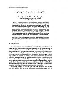
4.3 Data analysis Based on Table 1 we created the Burt’s Table (see Appendix). The application of multiple correspondence analysis showed that the total inertia explained is equal to 1.500 (percent of inertia: 12% is due to the first axis and 11% due to the second axis). A visualization of the results is presented in Figure 1. As we can see the profiles of cardiac patients (group 1) and controls (group 0) are quite different, as it was expected. In particular, presence of hypercholesterolemia (hchol 1), hypertension (htn 1), diabetes mellitus (dm 1), depression (depre 1), smoking status (smoki 1), male sex (sex 1), low education (educ 1), and physical inactivity (exerc 0) seems to characterize the patients group (group 1), since the distances in the factorial design are smaller than the other variables. On the other hand, subjects in the disease free group (group 0) are characterized by the absence of hypercholesterolemia (hchol 0), hypertension (htn 0), diabetes mellitus (dm 0), depression (depre 0), as well as the presence of middle to higher education (educ 2, educ 3). Now according to the contributions of the investigated parameters on the principal axis, we can see (see Appendix) that the first dimension include, beyond the study group, the classical cardiovascular risk factors (i.e., smoking habit, hypertension, hypercholesterolemia, diabetes mellitus) as well as an emerging risk factor (i.e., presence of depression), while the second dimension include physical activity and educational level, which seems to be secondary risk factors for the development of the disease in the investigated group. Moreover the parametric association model used in this work is the multinomial logit, described below:
Constant + GROUP + GROUP*DM + GROUP*EDU GROU + GROUP*HCHOL + GROUP*HTN + GROUP*PH ACTIV + GROUP*SEX + GROUP*SMOKING
The analysis showed that the previous model fits the data well since the chisquare for the likelihood ratio was found equal to 197.34 (d.f. = 183) and the significance is well above 5% (Type-I error = 0.220). In Table 2 we present selected results from the applied log-linear analysis. As we can see, hypercholesterolemia triples the risk (odds ratio = elog-odds) of developing coronary heart disease (log-odds = 1.2, 95% confidence interval 0.98 - 1.42), hypertension twofold the risk of developing the disease (log-odds = 0.76, 95% confidence interval 0.52 - 0.99), while physical activity prevents the development of coronary disease by reducing the relative risk by 22% (log-odds = -0.33, 95% confidence interval (−0.56, −0.10). However, the introduced model explains only the 16% of the total dispersion (source of dispersion due to model
82
D. B. Panagiotakos and C. Pitsavos
Table 2: Selected results from the log-linear analysis; analysis of dispersion Source of Dispersion Due to Model Due to Residual Total Parameter Hypercholesterolemia Hypertension Physical activity
Entropy
Concentration
d.f.
181.4792 957.0186 1138.4978
166.8671 653.3271 820.1942
8 1639 1647
log-odds
Standard error
Z-value
Asymptotic 95% confidence interval
1.20
0.11
10.61
(0.98, 1.42)
0.75 −0.33
0.12 0.12
6.40 −2.81
(0.52, 0.99) (−0.56, −0.10)
/ total = 181.47 / 1138.49). The previous results were, also, confirmed by the application of multiple correspondence analysis mentioned above (Figure 1). 5. Discussion In this work we presented a combined analysis of categorical data, using multiple correspondence analysis and log-linear models. It is widely adopted that by the application of multi correspondence analysis we can visualize the associations between the investigated (exposure) parameters and the disease. Therefore, applying correspondence analysis we can reduce the interaction parameters that are necessary for the classical log-linear models. Beyond the better understanding of the structure of the data the computational time may be significantly reduced. Moreover the graphical interpretation of the data that shows approximations of log-multiplicative parameters could be a useful tool in an exploratory epidemiological research, especially in the investigation, and, potentially, the reduction, of the level of the associations between the investigated parameters (interactions). Finally, interpreting the results from a public health perspective, epidemiologists could find inherent associations between the investigated variables and, consequently, design their policies with a more efficacious way. For example, in our data we can see that • middle aged participant with academic education are closely related to smoking habits
Interpretation of Epidemiological Data
83
2.0
1.5
AGEGROUP:75 -2.0
-2.5 -2.0
-1.5
-1.0
-0.5
0.0
0.5
1.0
1.5
2.0
Dimension 1
Figure 1: Correspondence Analysis for Table 1
• depression is closely related to the presence of hypercholesterolemia and the development of the disease These associations, and more other that can be found viewing the data should be taken into account, as interaction terms, for the fitting of log-linear models. This will enhance the analytical procedure and the interpretation of the data. Although, it is suggested that association model (i.e., log-linear) and correspondence analysis are highly related (Benzecri, 1973, Van Der Heijden, 1989, Blasius, 1994, Greenacre, 1994), the faintness of inference of correspondence analysis at population level limits the findings, only, to the observed data. References Andersen E. B. (1980). Discrete Statistical Models with Social Science Applications. North Holland. Benzecri J. P. (1973). Analyse des Donnees, vols 1 and 2. Dunod. Blasius J. and M. Greenacre. (1994). Computation of correspondence analysis. In
84
D. B. Panagiotakos and C. Pitsavos Correspondence Analysis in the Social Sciences – Recent Developments and Applications (Edited by M. Greenacre and J. Blasius). Academic Press.
Goodman L. A. (1986). Some useful extensions of the usual correspondence analysis approach and the usual log-linear models approach in the analysis of contingency tables. Int. Stat. Rev. 54, 243-309. Goodmann L. A. (1981). Association models and the bivariate normal for contingency tables with ordered categories. Biometrika 68, 347 - 355. Greenacre M. J. (1984). Theory and applications of correspondence analysis. Academic Press. Greenacre, M. J. (1994). Multiple and joint correspondence analysis. In Correspondence Analysis in the Social Sciences - Recent Developments and Applications (Edited by M. Greenacre and J. Blasius). Academic Press. Panagiotakos, D. B, Pitsavos, C., Chrysohoou, C., Moraiti, A., Stefanadis. C. and Toutouzas, P. K. (2001). The effect of short-term depressive episodes. In The Risk Stratification of Acute Coronary Syndromes: A Case-Control Study in Greece (CARDIO2000). Acta Cardiol 56, 357 - 365. Panagiotakos, D. B., Pitsavos, C., Chrysohoou, C., Stefanadis, C, and Toutouzas P. K. (2001). Risk stratification of coronary heart disease through established and emerging lifestyle factors. In A Mediterranean Population: CARDIO2000 Epidemiological Study. J. Cardiovasc. Risk 6, 329-335. Pitsavos, C., Panagiotakos, D. B., Chrysohoou, C., Skoumas, J., Stefanadis, C. and Toutouzas, P. K. (2002). How can education affect the risk of developing acute coronary syndromes? Results from CARDIO2000 epidemiological study. Bull World Health Organ 80, 371-377. Van der Heijden, P., De Falguerolles, A. and De Leeuw, J. (1989). A combined approach to contingency table analysis using correspondence analysis and log-linear analysis. App. Stat. 38, 249-292.
Interpretation of Epidemiological Data
85
Appendix. Burt Table Column Coordinates and Contributions to Inertia Input Table (Rows × Columns): 25 × 25 Total Inertia=1.5000 Table 3: Selected results from the log-linear analysis; analysis of dispersion (a) (1) (2) (3) (4) (5) (6) (7) (8) (9) (10) (11) (12) (13) (14) (15) (16) (17) (18) (19) (20) (21) (22) (23) (24) (25)
1 2 3 4 5 6 7 8 9 10 11 12 13 14 15 16 17 18 19 20 21 22 23 24 25
(b)
(c)
(d)
(e)
(f)
(g)
(h)
(i)
(j)
−1.50 1.33 .001 .032 .066 .010 .018 .008 .014 −.935 .940 .007 .128 .062 .032 .064 .036 .064 −.520 .615 .021 .173 .053 .031 .072 .048 .101 −.029 .157 .029 .010 .047 .000 .000 .004 .010 .502 −.361 .036 .219 .042 .050 .144 .028 .075 .173 −1.96 .006 .248 .063 .001 .002 .138 .246 −.138 .274 .081 .402 .013 .008 .082 .036 .320 .589 −1.167 .019 .402 .054 .036 .082 .155 .320 −.557 −.370 .056 .581 .029 .095 .403 .046 .178 .724 .481 .043 .581 .038 .123 .403 .060 .178 .126 −.429 .061 .318 .026 .005 .025 .068 .293 −.200 .683 .038 .318 .041 .008 .025 .108 .293 −.455 .025 .065 .380 .024 .072 .378 .000 .001 .832 −.045 .035 .380 .043 .132 .378 .000 .001 −.438 −.320 .059 .419 .028 .061 .273 .036 .146 .623 .455 .041 .419 .039 .087 .273 .051 .146 −.258 −.038 .083 .333 .011 .030 .326 .001 .007 1.265 .184 .017 .333 .055 .147 .326 .003 .007 −.125 −.177 .075 .142 .0166 .006 .047 .014 .095 .377 .535 .025 .142 .051 .019 .047 .043 .095 .178 −.603 .032 .184 .045 .005 .015 .069 .170 .098 .201 .052 .053 .032 .003 .010 .012 .043 −.645 .530 .016 .138 .056 .037 .083 .028 .056 .025 −.070 .061 .008 .026 .000 .001 .002 .007 −.038 .108 .039 .008 .040 .000 .001 .003 .007
(a)=row number, (b)=coordinate dimension 1, (c)= coordinate dimension 2, (d)=Mass, (e)=Quality, (f)=Relative inertia, (g)= Inertia dimension 1, (h)=Cosine2 dimension 1, (i)= Inertia dimension 2, (j)=Cosine2 dimension 2; (1)= AGEGROUP:< 35, (2)=AGEGROUP:35-45, (3)= AGEGROUP:45-55, (4)=AGEGROUP:55-65, (5)=AGEGROUP:65-75, (6)= AGEGROUP:> 75, (7)= SEX:Aνδρεζ, (8)= SEX:Γυνακε, (9)= GROUP:Normals, (10)=GROUP:CHDpati, (11)=SMOKING:No-smoke, (12)= SMOKING:Smoker, (13)= HTN:Normal, (14)= HTN:Hyperten, (15)= HCHOL:Normal, (16) = HCHOL:Abnormal, (17)= DM:Normal, (18)= DM:Diabetic, (19)= SIG DEPR:0, (20)= SIG DEPR:1, (21)= EDU GROU:1, (22)= EDU GROU:2, (23)= EDU GROU:3, (24)= PH ACTIV:No, (25)= PH ACTIV:Yes.
Received June 14, 2002; accepted November 29, 2002
86
D. B. Panagiotakos and C. Pitsavos
Demosthenes B. Panagiotakos Biostatistician-Epidemiologist/Lecture A’ Cardiology Clinic, School of Medicine University of Athens, Greece 46 Paleon Polemiston Street 166-74 Glyfada, Attica, Greece
[email protected] Christos Pitsavos Department of Cardiology, School of Medicine University of Athens, Greece