Interpreting Genotype by Environment Interaction Using ... - Core

Statistics and Applications Volume 10, Nos. 1&2, 2012 (New Series), pp. 45-62

Interpreting Genotype by Environment Interaction Using Weather Covariates Roma Rani Das1, Anil Kumar V. 1, Sujay Rakshit2, Ravikanth Maraboina1, Sanjeev Panwar3, Seema Savadia4 and Abhishek Rathore1 1 International Crops Research Institute for the Semi-Arid Tropics, Patancheru, India 2 Directorate of Sorghum Research, Rajendranagar, Hyderabad, India 3 Indian Agricultural Statistics Research Institute, Pusa, New Delhi, India 4 National Environmental Engineering Research Institute, Nehru Marg, Nagpur, India ________________________________________________________________________ Abstract Understanding genotype by environment interaction (G*E) has always been a challenge to statisticians and plant breeders. Recently site regression analysis has emerged as a powerful analysis tool to understand G*E, specific and general adaptability of genotypes and grouping of environments into mega-environments. This paper attempts to enhance power of site regression by using environmental covariates in tandem to explain G*E better. In this present study, performances of eighteen genotypes were investigated across five environments during the year 2008 rainy season. Three traits, namely grain yield, harvest index and dry fodder yield were used for analysis purpose. Biplot analysis identified two major groups of environments, first group of environments included Karad and Coimbatore and second group consisted Udaipur, Palem and Surat. SPH 1615 and SPH 1609 were identified as winning genotypes for first megaenvironment whereas SPH 1596, SPH 1611 and CSH 16 were winners for second megaenvironment for grain yield. High yielding genotypes, SPH 1606, SPH 1616 and CSH 23 performed consistently well across all environments and should be considered for general adaptability. Genotype SPH 1596 was identified for both specific and general adaptability. By superimposing GGE biplots for different traits, genotypes SPH 1596 and CSH 23 were identified as stable for all three traits. Climatic data on average maximum temperature and minimum temperature at early (June-July) and late phase (August) of plant growth was incorporated to study G*E by using factorial regression. Average maximum temperature and minimum temperature at early phase and average minimum temperature during late phase were found significantly affecting genotype performance.

46

ROMA RANI DAS ET EL.

[Vol.10, Nos. 1&2

Genotypic sensitivities for each genotype were estimated. Genotype SPH 1606 with negative genotypic sensitivity was found to perform better in Karad with below average maximum temperature during early phase. Genotype CSH 16 with negative genotypic sensitivity for average minimum temperature during early phase and positive genotypic sensitivity average minimum temperature during late phase performed better in Palem. Keywords: AEA (Average Environment Axis); biplot; Factorial regression; G*E (Genotype by Environment interaction); GGE (Genotype plus Genotype by Environment); MET (Multi-Environment Trial); PCA (Principal Component Analysis); stability, Site regression; SVD (Singular Value Decomposition). _______________________________________________________________________

1

Introduction

Releasing genotypes from breeding programs suffers primarily due to variability present in target environments and their interaction with breeding material. Understanding the performance of genotypes over diverse environments has always been an important goal and challenge before plant breeding community. To understand this, usually Multi-Environment Trials (MET) are planned and data from several environments and/or years are gathered systematically. Various statistical models are used to study genotype by environment interaction (G*E). If a statistical model is able to explain pattern of G*E to a meaningful extent, genotypes are released accordingly. However, in most cases this task is not easy and straightforward and need lots of exploration of data. Since early 1960s several efforts were made by various researchers to explain G*E by use of different statistical models. Towards this direction initial efforts were mainly centered towards using regression based approaches. Most commonly regression based stability models were given by Wricke (1962), Finlay and Wilkinson (1963), Eberhart and Russell (1966), Perkins and Jinks (1968), Freeman and Perkins (1971), Shukla (1972) and Franchis and Kannenberg (1978). Out of these Eberhart and Russell (1966) stability model has been exploited by breeders widely. Their model assumes that the genotypes have a linear response to change with environments. According to this model, a genotype is said to be stable having high mean yield, with coefficient of regression (bi) equal to one and deviation from linear regression(Sdi2) equal to zero. Wricke (1962) suggested using G*E for each genotype as a stability measure, which is termed as ecovalence (Wi2). Shukla (1972) presented a statistic called stability variance (σi2) that partitions G*E and assigns it to individual genotype. Franchis and Kannenberg (1978) used the environmental variance (Si2) and the coefficient of variation (CVi) to define a stable genotype. Soon it was realized that G*E pattern always cannot be explained by using additive models and hence another important milestone in studying G*E was introduction of multiplicative models (Zobel et al., 1988) and use of biplots (Gabrial, 1971). Biplots

2012]

INTERPRETING GENOTYPE BY ENVIRONMENT INTERACTION

47

are used to graphically summarize G*E pattern mostly on a two-dimensional graph, depicting relationship between genotypes and environments. This graphical representation has been found extremely helpful in selecting specific and generally adapted genotypes. Two types of biplots, the AMMI biplot (Crossa et al., 1990 and Gauch, 1992) and the GGE biplot (Yan et al., 2000; Yan and Kang, 2003; Joshi et al.,2007) are the most commonly used biplots. Two dimensional biplots apply multivariate techniques such as Singular Value Decomposition (SVD) to approximate multidimensional information into two dimensions to address the issue of genotype recommendation in multi-environment trials through graphical visualization. To strengthen genotype recommendation, a usual practice among breeders is to repeat trial over years and revalidate recommendations again. In this approach many times because of change in climatic conditions at specific environment, crossover (Yang, 2007) kind of G*E are observed frequently, which makes it difficult to take decision for genotype adaptability. Biplots over multiple years and environments may be useful for such situations, however many time this becomes very difficult to give recommendations and also to understand change in performance of genotypes. To understand such behavior one may use techniques where data on various environmental variables which are supposed to influence genotype performance like temperature, precipitation, sunshine, relative humidity and other important weather parameters are carefully recorded. Once such information is available one may try to explain performance of specifically adapted genotypes to individual environments based on these climatic parameters. Such studies come under a wider class of techniques named factorial regression (Eeuwijk et al., 1966). Factorial regression with environmental covariates has been proved extremely helpful in understanding G*E relation to environmental covariates (Voltas et al., 2005). In factorial regression, environment variables are tested for their possible association with the genotypes performance across environments. Once these variables are identified it becomes easier and more confident to recommend genotypes for specific adaptation. In addition to above breeders are often more interested in studying common stability of various traits together to screen and recommend genotypes to targeted regions. The objective of the present study is also to identify adaptable genotypes for targeted environments by using weather covariates and use of multiple traits.

2

Material and Methods

Experimental material and environment - Data used for this study was taken from All India Coordinated Sorghum Improvement Project, where eighteen genotypes were evaluated under Advanced Varietal and Hybrid Trial (AVHT) during the year 2008 rainy season. Experiment was conducted at nineteen environments across India, however five

48


[Vol.10, Nos. 1&2

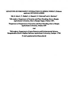
environments viz., Coimbatore (COIM), Karad (KARA), Palem (PALE), Surat (SURA) and Udaipur (UDAI) were considered for study as consistent environmental weather data was available for these environments. These environments mainly covered the western and southern-east region of India (Fig 1). The materials included 10 test hybrids, 2 test varieties, 2 hybrid checks (CSH 16, CSH 23), 3 variety checks (SPV 1616, SPV 462, CSV 15) and to these one absolute check was also included. Details of the genotypes are presented in Table 1. Detail information on environments relative to area/state, latitude, longitude, altitude, date of sowing and harvesting is given in Table 2. The experimental design at each environment was a randomized complete block design with eighteen genotypes replicated thrice. Field management practices such as application of fertilizers and use of pesticides were standard across all environments. Planting started during middle of June and ended by the first week of July across all environments. Data were recorded on grain yield (GY) and dry fodder yield (DFY). Another statistic, harvest index (HI) was calculated as the ratio of grain mass to total above ground biomass and was used to measure the proportion of grain yield value to total biomass collected and was used for analysis purpose. Grain yield ranged from 1456 kg/hectare to 6311 kg/hectare and dry fodder yield ranges from 3704 kg/hectare to 22072 kg/hectare across five environments. Table 1: Information on the genotypes used in the study Genotype Genotyp Contribut s Names es Code ing sector SPH 1596 G1 Private SPH 1603 G2 Private SPH 1604 G3 Private SPH 1605 G4 Public SPH 1606 G5 Private SPH 1609 G6 Private SPH 1610 G7 Private SPH 1611 G8 Private SPH 1615 G9 Private SPH 1616 G10 Private SPV 1616 G11 Public SPV 1786 G12 Public SPV 1817 G13 Public SPV 462 G14 Public CSH 16 G15 Public CSH 23 G16 Public CSV 15 G17 Public Absolute Fig 1. Geographical position of the trial G18 Check environmentsinvolved in study

2012]


49

Table 2: Information on the trial environments Environments (Code) Coimbatore (COIM) Karad (KARA) Palem (PALE) Surat (SURA) Udaipur (UDAI)

Area/States

Latitude

Longitude

Date of sowing

Date of harvest

76° 59' 00" E

Altitude (msl) 412

Tamil Nadu

11° 02' 00" N

16th June 2008

04th Oct 2008

Maharashtra

17° 16' 26" N

74° 17' 02" E

597

29th June 2008

08th Oct 2008

Andhra Pradesh Gujarat

16° 35' 00" N

78° 00' 00" E

642

28th June 2008

27th Oct 2008

21° 11' 45" N

72° 49' 52" N

1340

08th July 2008

26th Oct 2008

Rajasthan

27° 42' 00" N

75° 33' 00" E

598

01st July 2008

15th Oct 2008

Statistical Analysis - Analysis of variance was carried out for grain yield using proc glm procedures of SAS software version 9.3 for Windows (SAS Institute Inc., 2008). To pool data, homogeneity of error variance across five environments was tested using Bartlett test (Gomez and Gomez, 1984) and the chi-square statistic was found significant. Aitken’s transformation was used to make error variances homogeneous. In order to determine the contribution of environment, genotype and their interaction following statistical model was used: Y ijk = µ + g i + e

j

+ r jk + ( ge ) ij + ε ijk

is the yield of genotype i in block k for environment j, µ is the grand mean, th th th gi and e j are the main effects of i genotype and j environment respectively, r jk is the k

where,

Yijk

replicate effect in jth environment, (ge)ij is the interaction effect between ith genotype and jth environment and ε ijk is the error effect. Site regression (GGE) using Biplot - A standard biplot is the scatter plot that graphically displays both the row factor and column factors of a two-way table data. A biplot graphically displays a matrix with application to principal component analysis (Kroonenberg, 1995). For generating a biplot, a two-way table representing two factors was subjected to singular value decomposition. The singular value decomposition of a matrix X= ( x ij )vxs is given by r

xij = ∑uik λk vkj k =1

where, ( uik ) is the element of the matrix Uvxs characterizing rows, λk ’s are the singular values of a diagonal matrix Lsxs, v kj is the element of the matrix Vsxs characterizing the columns and r represents the rank of matrix X≤min(v,s). Principal component scores for

50


[Vol.10, Nos. 1&2

row and column factors were calculated after singular value partitioning of ( xij )vxs (Yan et al., 2002). Biplot was obtained using first two components and percentage of variation explained by them is calculated. The fixed effect two-way model for analysing multi-environments genotype trials is as follow: E ( Y ij ) = µ + g i + e j + ( ge ) ij

where, µ is the grand mean, gi and e j are the genotype and environmental main effects respectively, ( ge ) ij is the G*E effect. The sites regression model is given by (Crossa and Cornelius, 1997; Yan and Kang, 2003): r

*

E(Yij ) = µ + e j + ∑ξin η jn

*

n=1

where, r = number of principal components (PCs) required to approximate the original *

*

data. ξin and η jn are the ith genotype and the jth environmental scores for PCn, respectively. In the site regression method, PCA is applied on residuals of an additive model with environments as the only main effects. Therefore, the residual term r

∑ξ

* in

η jn* contains the variation due to G and G*E. A two dimensional biplot (Gabriel,

n =1

1971, Parsad et.al, 2007) derived from above 2-way table of residuals is called GGE biplot (G plus G*E) (Yan et al., 2000). A GGE biplot graphically depicts the genotypic main effect (G) and the G*E effect contained in the multi-environment trials. GGE biplots have been found very useful in understanding G*E, mega environment identification and genotype recommendation. All five environments data was fitted using site regression model and which-won-where and ranking biplot were generated. Factorial Regression - For better understanding of G*E pattern, inclusion of environmental covariates into study is always useful. The most common technique to explain G*E by environmental covariates is factorial regression. The general form for a factorial regression model with H environmental covariates is given by (Denis, 1988; Van Eeuwijk et al., 1996): H

E(Yij ) = µ + gi + e j + (∑βih E jh + δij ) h =1

where β ih to βiH are sensitivities of ith genotype to environmental variables E1 to EH, H being the number of covariates included in the model and δij is the component of deviation from regression.

2012]


51

After fitting the main effects  , gi , and e j , environmental variables are included on the H

levels of environmental factor to describe the G*E interaction as geij = ∑ β ih E jh + δ ij h =1

Now the geij effect for each genotype i, can be regressed on to environmental covariates Eh (h = 1 to H) to obtain the sensitivity coefficients for that genotype .A usual way of determining weather covariates influencing genotype performance is to fit factorial regression model by fitting all possible linear models and are select best combination by using some statistical criteria. A commonly used method for selection of best model in factorial regression is Mallows’ Cp selection criteria and adjusted R-square value (Draper and Smith, 1981). After fitting the main effects µ , gi and e j , the environmental variables are introduced in an attempt to describe G*E interaction by fitting of regression line for individual genotype corresponding to environmental variables that resulted in estimation of genotypic sensitivities. During present study four weather covariates were included and Mallows’ Cp selection criteria were used for selecting significant covariates. Selected covariates were standardized to facilitate interpretation and the genotypic sensitivities were estimated by least square method.

3

Results and Discussions

Analysis of Variance and study of crossover type of G*E Homogeneity test for error variance was computed to pool multi-environments trial data with five environments and 18 genotypes for grain yield using Bartlett chi-square test. Bartlett test resulted in a highly significant chi-square value (χ2 =55.04**). Hence, data were transformed to make error variance homogeneous. Transformed data was analyzed using analysis of variance technique (Table 3). All sources of variation (i.e., due to E, G and G*E) were found to contribute significantly towards yield variation. The total amount of variation (i.e., E+G+G*E) accounted by environment (E), genotype (G) and genotype by environment interaction (G*E) were 88.21%, 5.64% and 6.15%, respectively. Mean plot (Fig 2) of genotypes across environments was drawn to visualize the ranking of genotypes based on yield performance. The rank of genotypes was changing across environments, which suggested existence of crossover G*E.

52


[Vol.10, Nos. 1&2

Table 3: Combined Analysis of Variance of grain yield data (transformed) of 18 genotypes tested across 5 environments Source of Variation Environment Genotype Genotype * Environment CV (%): 12.46

Degrees of Freedom 4 17 68 R2: 0.97

Mean Square Error 1129.60** 16.99** 4.64**

Proportion of (E+G+G*E) 88.21 5.64 6.15

**denotes significance at p