Intersecting hyper-surfaces in dimensionally continued topological ...

Intersecting hypersurfaces in dimensionally continued topological density gravitation

arXiv:hep-th/0306220v4 25 Aug 2004

Elias Gravanis,

Steven Willison

Department of Physics, King’s College London, Strand, London WC2R 2LS, United Kingdom. Abstract We consider intersecting hypersurfaces in curved spacetime with gravity governed by a class of actions which are topological invariants in lower dimensionality. Along with the Chern-Simons boundary terms there is a sequence of intersection terms that should be added in the action functional for a well defined variational principle. We construct them in the case of Characteristic Classes, obtaining relations which have a general topological meaning. Applying them on a manifold with a discontinuous connection 1-form we obtain the gravity action functional of the system and show that the junction conditions can be found in a simple algebraic way. At the sequence of intersections there are localised independent energy tensors, constrained only by energy conservation. We work out explicitly the simplest non trivial case.

Introduction General relativity can be generalised to a manifold with boundary. The inclusion of a certain boundary term (Gibbons-Hawking) makes the action principle well defined on the boundary. Also, singular hypersurfaces of matter[1] can be incorporated into a manifold with piece-wise differentiable metric[2]. We will see that these are part of the general properties of actions built out of dimensionally continued topological invariants. The Einstein-Hilbert action of General Relativity is the dimensionally continued form of the two dimensional Euler Characteristic. A linear combination of terms which are dimensionally continued Euler densities in arbitrary dimensions is known variously as Lovelock or Lanczos-Lovelock or Gauss-Bonnet gravity. It has been studied extensively[3, 4, 5, 6] and the boundary action has been constructed[7, 8, 9]. An interesting problem in gravity is the study of collisions of shells of matter[10, 11, 12]. Brane-world models of matter on the intersection of co-dimension 1 branes were studied and it was found that the Gauss-Bonnet term was needed in order to get a tension on the intersection in a natural way[13]. The Gauss-Bonnet term is the dimensionally continued 4-dimensional Euler density. We address this problem of intersections and collisions of co-dimension 1 hypersurfaces in a more generalised way, motivated by the properties of the topological invariants. A topological invariant ‘action’ contains no local degrees of freedom. The only information it encodes is topological. As such it is independent of the local form of the metric.

1

We consider actions which are topological in a certain dimensionality and then generalise to higher dimensions. These actions have the property that the independent infinitesimal variation of the action with respect to the connection is a total derivative. We consider a smooth manifold with embedded arbitrarily intersecting hypersurfaces of singular matter. We can view a hypersurface as the shared boundary of two adjacent regions. The gravity of localised matter can be described by a boundary action. As in [13], we allow for the possibility of matter being localised on the surfaces of intersection also. The spacetime is divided up into polyhedral regions bounded by piece-wise smooth hypersurfaces- like a matrix of cells. We show that this situation is compatible with any theory of gravity based on a dimensionally continued topological invariant. We exploit the topological nature of the theory to write the action in terms of different connections in different regions. This generates our surface actions remarkably simply. We can derive the Israel junction conditions and the junction conditions for any intersections in a purely algebraic way. In section 1 we review basic material on topological densities, introducing Characteristic Classes on a manifold with boundary. In section 2.1 we derive the intersection forms generalising Chern-Simons forms and in section 2.2 we construct the action functional of gravity in the presence of intersecting hypersurfaces employing the properties of the intersection forms. The topological theory is dealt with in section 2.2.1 and the dimensionally continued case of interest is dealt with in section 2.2.2. In section 3 we work out a simple example along with the energy exchange relations in that case.

1

Topological densities and gravitation

Let M be a manifold with a Riemannian or Lorentzian metric g and a Levi-Civita connection. Let ω be the connection 1-form and Ω the curvature form. For dimM = 2n consider the integral Z f (Ω, ..Ω), f (Ω, .., Ω) = Ωa1 a2 ∧ ... ∧ Ωa2n−1 a2n ǫa1 ...a2n (1) M

where ǫ... is the fully anti-symmetric symbol and ǫ1..2n = +1 and the integral is assumed to exist. The frame E is ortho-normal in the sense g(E a, E b ) = δ ab in the Riemannian case and g(E a , E b ) = η ab = diag(−1, 1..1) in the Lorentzian case. When g is Riemannian and M is compact and oriented f (Ω, ..Ω) represents the Euler class. The integral over M, normalised properly, gives the Euler number of M, according to the renowned Gauss-Bonnet-Chern Theorem[14]. There are more general (and precise) definitions than the one we give here. The details are in the textbooks[15, 16, 17] but we only need to point out the similarity and make intelligible borrowing of tools from global differential geometry. f (Ω, ..Ω) will be called the Euler density. In general an invariant whose integral over M gives a topological invariant of M will be called topological density. Let us now repeat the Chern-Weil construction and show that under a continuous change of the connection, ω → ω ′ , f (Ω, ..Ω) changes by an exact form. In fact we are only 2

going to need f to be invariant, symmetric and multi-linear. These general properties are provided by the invariant polynomials and lead to the so-called Characteristic Classes, of which the Euler class is an example. The following applies globally on the principal bundle but it is sufficient for our purpose to work on the manifold. Define ωt = tω + (1 − t)ω ′ Call θ = ω − ω′ and note that θ=

d ωt dt

and for the curvature associated with ωt Ωt = dωt + ωt ∧ ωt

(2)

that

d Ωt = Dt θ (3) dt where Dt is the covariant derivative associated with ωt . Then Z 1 Z 1 d ′ ′ f (Ω, .., Ω) − f (Ω , .., Ω ) = dt f (Ωt , .., Ωt ) = n dtf (dΩt /dt, Ωt , ...Ωt ) = (4) dt 0 0 Z 1 Z 1 =n dtf (Dt θ, Ωt , ...Ωt ) = n dt df (θ, Ωt , ...Ωt ) 0

0

where symmetry and multi-linearity of f have been used, as well as Dt Ωt = 0. If we define L(ω) = f (Ω, ..Ω) and ′

L(ω, ω ) = −n

Z

(5)

1

dtf (ω − ω ′ , Ωt , ...Ωt )

(6)

0

we can write L(ω) = L(ω ′) − dL(ω, ω ′)

(7)

Now, assume that, for example, M is non-compact and without a boundary. If L(ω, ω ′) vanishes fast enough asymptotically Z L(ω) (8) M

(assumed to exist) does not depend on ω. It is this property that makes L(ω) so useful when, with a little modification, it is used as a Lagrangian for gravity for dimM > 2n. Define the (d-r)-form (which is a natural (d-r)-dimensional volume element): ea1 a2 ...ar =

1 ǫa a ...a E ar+1 ∧ .. ∧ E ad . (d − r)! 1 2 d 3

(9)

The associated dimensionally continued Euler density for d > 2n is Lg (ω, e) = f (Ω, .., Ω, e) = Ωa1 b1 ∧ Ωa2 b2 ∧ .. ∧ Ωan bn ∧ ea1 b1 a2 b2 ...an bn which is also an invariant. Then, the Euler-Lagrange variation with respect to ω in Z Lg (ω, e),

(10)

(11)

M

noting that δΩ = D(δω), vanishes by the Bianch identity and the assumed zero torsion condition DE a = 0[18]. The equations of motion are obtained simply by the Euler-Lagrange variation of the frame, applying the formula δea1 ..ar = δE ar+1 ∧ ea1 ..ar ar+1

(12)

in a purely algebraic way. In the next section we find how the action (10) is re-expressed in the presence of hypersurfaces and their intersections, by generalising (7) appropriately, and show that the equations of motion (junction conditions) are still obtained from the mere variation of the frame.

2

Topological densities on manifolds containing intersecting hypersurfaces

A hypersurface is understood as a smooth co-dimension 1 subspace of the manifold where the connection form exhibits discontinuity or as a (higher co-dimension) intersection of such discontinuities. Integrating L(ω) over the manifold, when ω is the discontinuous connection form, one has to add a Chern-Simons term integrated over the discontinuity for the final result to have well defined variations with respect to ω (and to be diffeomorphism invariant). If discontinuities intersect, in all possible ways, one should, in general, add appropriate generalisations of the Chern-Simons forms integrated over the intersections. A discontinuity can be thought of as the common boundary of two d-dimensional (bulk) regions. Intersection of discontinuities can be thought of as common subspaces of the (not smooth) boundaries of a larger number of bulk regions. It is also helpful to think of them as singular overlaps (at the boundaries) or intersections of two or more bulk regions. With this in mind, we first find generalisations of the Chern-Simons forms.

2.1

From boundary to intersection action terms

Given an invariant polynomial, we found in the previous section a relation of the form of (7) by interpolating between the given connection ω and an arbitrary one ω ′ . We can 4

continue by interpolating between the latter and a new connection. In general, let us define the p-parameter family of connections, interpolating between p+1 connections, ω 1 , .., ω p+1, ωp = ωt1 ..tp = ω 1 − (1 − t1 )θ1 − ... − (1 − t1 )..(1 − tp )θp

(13)

where θr = ω r − ω r+1 ,

r = 1, .., p.

(14)

Note: For the purposes of section 2.1 and equations 38 to 44 only, the subscript p refers to a function of t1 , ...tp . Define p

X ∂ ∂ (1 − t1 )..(1\ − tq )...(1 − tr )θr = θtq ...tbq ...tp = θpq . ωp = ωt1 ..tp = 1 ∂tq ∂tq r≥q

(15)

where the hat means that the index is omitted. Note that ωt1 ..tp |tr =0 = ωt1 ..tr−1tr+1 ..tp

(16)

setting the connection ω r = 0. This will be useful below. Let Ωp be the p-parameter curvature 2-form associated with ωp . Then ∂ ∂ Ωp = Ωt ..t = Dt1 ..tp θtq ...tb ...t = Dp θpq . q p 1 ∂tq ∂tq 1 p

(17)

There is also a “Bianchi identity” for Ωp Dp Ωp = 0

(18)

Dp is the covariant derivative associated with ωp . Proposition 1. We introduce a (p+1)-point term with p+1 connection entries. We now show that the (p+1)-point generalization of the 2-point Chern-Simons term takes the form Z 1 n! 1 p+1 dt1 ..dtp f (θp1 , θp2 , ..θpp , Ωp , ..Ωp ) (19) L(ω , .., ω ) = ηp (n − p)! 0 where ηp = (−1) p+1 X s=1

p(p+1) 2

. These terms obey the following rule:

(−1)s−p−1 L(ω 1, .., c ω s , .., ω p+1, ω p+2) = L(ω 1 , .., ω p+1) + dL(ω 1, .., ω p+1, ω p+2).

(20)

Proof: If we define ωtp+1 = tp+1 ω p+1 + (1 − tp+1 )ω p+2 p+1 5

(21)

then L(ω

1

, .., ωtp+1 ) p+1

n! = ηp (n − p)!

Z

1

p 1 2 dt1 ..dtp f (θp+1 , θp+1 , ..θp+1 , Ωp+1 , ..Ωp+1 )

0

We have Z

1 ∂ L(ω 1, .., ω p , ωtp+1 ) L(ω , .., ω , ω ) − L(ω , .., ω , ω ) = dtp+1 p+1 ∂t p+1 0 Z 1 n! ∂ p 1 2 = ηp f (θp+1 , θp+1 , ..θp+1 , Ωp+1 , ..Ωp+1 ) dt1 ..dtp dtp+1 (n − p)! 0 ∂tp+1 1

p

1

p+1

p

p+2

From the multi-linearity of the invariant polynomial f we have ∂ p 1 2 , Ωp+1 , ..Ωp+1 ) = f (θp+1 , θp+1 , ..θp+1 ∂tp+1 p X ∂ r p 1 f (θp+1 , .., θp+1 , .., θp+1 , Ωp+1 , ..Ωp+1 ) + ∂tp+1 r=1 p 1 2 , (n − p)f (θp+1 , θp+1 , ..θp+1

∂ Ωp+1 , ..Ωp+1 ) ∂tp+1

Using (17) we can write the last term as p p+1 1 2 (n − p)(−1)p df (θp+1 , θp+1 , ..θp+1 , θp+1 , Ωp+1 , ..Ωp+1 ) p X p+1 s (−1)p+s−1 f (θp1 , .., Dp+1 θp+1 , .., θp+1 , Ωp+1 , ..Ωp+1 ) −(n − p) s=1

and using again (17) in the last term we obtain −

p X

(−1)p+s−1

s=1 p

+

X

(−1)

p+s−1

∂ p+1 1 s f (θp+1 , .., θd p+1 , .., θp+1 , Ωp+1 , ..Ωp+1 ) ∂ts p+1 X

1 f (θp+1 , ..,

r=1,6=s

s=1

∂ r p+1 p s θp+1 , ..θd p+1 , .., θp+1 , θp+1 , Ωp+1 , ..Ωp+1 ) ∂ts

In all p p+1 1 2 (n − p)(−1)p df (θp+1 , θp+1 , ..θp+1 , θp+1 , Ωp+1 , ..Ωp+1 ) p X ∂ p+1 1 s (−1)p+s−1 − f (θp+1 , .., θd p+1 , .., θp+1 , Ωp+1 , .., Ωp+1 ) ∂t s s=1

+

p+1 X s=1

p+s−1

(−1)

p+1 X

r=1,6=s

1 f (θp+1 , ..,

∂ r p p+1 s θ , .., θd p+1 , .., θp+1 , θp+1 , Ωp+1 , .., Ωp+1 ) ∂ts p+1 6

Note now that

∂ ∂ ∂ s ∂ r θp+1 = ωp+1 = θ (22) ∂ts ∂ts ∂tr ∂tr p+1 then in the last term, if we split the sum into r < s and r > s, changing variables r ↔ s in the latter and using this identity we see that the term vanishes. We have shown then that (p+1)-point Lp+1 defined in (19) obeys a rule p+1 X s=1

cs , .., ω p+1, ω p+2) = L(ω 1, .., ω p+1) + dL(ω 1, .., ω p+1, ω p+2) (−1)s−p−1 L(ω 1, .., ω

The relation (16) has been used.

It is not hard to show that L is fully anti-symmetric in its entries, so we can write the above in the form p+1 X

L(ω 1 , .., ω s−1, ω ′, ω s+1, .., ω p+1) = L(ω 1, .., ω p+1) + dL(ω 1, .., ω p+1, ω ′)

(23)

s=1

where ω ′ is arbitrary. As θr is a 1-form we have f (.., θr , .., θr , .., Ωp , ..Ωp ) = 0 and we can write (19) explicitly in terms of θr = ω r − ω r+1, r = 1..p in the form Z 1 1 p+1 L(ω , .., ω ) = dt1 ..dtp ζp f (θ1 , θ2 , ..θp , Ωp , .., Ωp ), (24) 0

ζp = (−1)

p(p+1) 2

p−1 Y n! (1 − tr )p−r . (n − p)! r=1

(25)

Let us show that Lp ’s, constructed from Characteristic Classes, are invariant under local Lorentz transformations. The connections transform as r ω(g) = g −1ω r g + g −1dg

(26)

for all r = 1, .., p + 1, where g belongs to the adjoint representation of SO(d-1,1). Then, r θ(g) = g −1θr g and Ωp(g) = g −1 Ωp g, so [20] p+1 1 , .., ω(g) ) = L(ω 1, .., ω p+1). L(ω(g)

(27)

In fact, one can derive (23) without reference to the invariant polynomial , by use of the Poincare lemma and the following observation (inspired by the form of (23)). If f (x1 , ..xn ) is an anti-symmetric function of n variables and Af (x1 , ..xp , xp+1 ) = f (x1 , ..xp ) −

p X i=1

7

f (x1 , .., xi−1 , xp+1 , xi+1 , ..xp )

(28)

(antisymmetrising over n+1 variables) then AAf (x1 , .., xp+2 ) = 0. The proof is trivial. We can now show (23) by induction assuming only that L(ω) obeys (7). I.e. it is true for the p=0 case. Assume (23) for p=k-1 (let us use the symbol Lk (ω 1 ..ω k ) for the intersection forms in this proof) ALk (ω 1 ..ω k+1) = −dLk+1 (ω 1 ..ω k+1)

(29)

Then dALk+1 (ω 1 ..ω k+2) = 0. By the Poincare lemma we have that there exists an invariant form, locally, such that ALk+1(ω 1 ..ω k+2) = −dLk+2(ω 1 ..ω k+2)

(30)

which completes the induction. (19) is a solution of the general relation (23). There is similarity between our composition rule and Stora-Zumino descent equations [21]. The reason is the existence in both cases of a nilpotent operator, A in our case and the fermionic BRST operator there, which commutes and anticommutes respectively with the derivative operator d.

2.2

Manifolds with discontinuous connection 1-form

We now construct the action functional of gravity on a manifold containing intersecting surfaces. It will also enable us to draw conclusions for arbitrary intersections of hypersurfaces for a general dimensionally continued topological density. 2.2.1

Topological density R If the functional M L is independent of the C 0 metric of the manifold M, then it can be evaluated using a continuous connection as well as a connection that is discontinuous at some subspaces (namely there are hypersurfaces involved). ThatR is, the result will be the same. We use this formal equivalence to give a meaning to M L(ω) when ω is discontinuous. Let us start with the case of a topological density L(ω0) of a continuous connection ω0 integrated over M which contains a single hypersurface. Label 1 and 2 the regions of M separated by the hypersurface. Introduce two connections, ω1 and ω2 which are smooth in the regions 1 and 2 respectively. We now write Z Z Z L(ω0 ) = L(ω1) + dL(ω1, ω0 ) + L(ω2 ) + dL(ω2 , ω0 ) (31) 1

M

2

R R Label the surface, oriented with respect to region 1, with 12. (Formally 12 = − 21 ). Z Z Z Z L(ω0 ) = L(ω1 ) + L(ω2 ) + L(ω1 , ω0 ) − L(ω2 , ω0 ) M 1 2 12 Z Z Z = L(ω1 ) + L(ω2 ) + L(ω1 , ω2 ) + dL(ω1, ω2 , ω0 ) (32) 1

2

12

8

3

{31}

{23} {123}

1 2 {12}

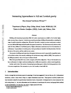
Figure 1: The simplicial intersection of co-dimension 2 (h=2). The totally antisymmetric symbol {123} specifies the intersection including the orientation

That is, for a smooth surface the r.h.s. is independent of ω0 . Consider now a sequence of co-dimension p = 1, 2, 3..h hyper-surfaces which are intersections of p + 1 = 2, 3..h + 1 bulk regions respectively. We will use the terms intersection and hyper-surface alternatively. A co-dimension p hyper-surface is labelled by i0 ..ip where i0 , .., ip are the labels of the bulk regions which intersect there. We call this configuration a simplicial intersection. We take the example h = 2 (fig. 2.2.1), where the intersections are {12}, {13}, {23}, {123}. An exact form integrated over {12} will contribute at {123} the opposite that when integrated over {21}, that is, for the latter integration the intersection can be labelled by −123 = 213, if we assume anti-symmetry of the label. The arrows of positive orientations in fig. 1 tell us that a fully anti-symmetric symbol {123} will adequately describe the orientations of the intersection 123. This is in contrast to the non-simplicial intersection (fig. 2.2.1). Definition 2 (for a simplicial intersection). {i0 ...ip } is the set i0 ∩ · · · ∩ ip where ir P is the closure of the open set ir (a bulk region). ir overlap such that ∂ir = hs=0,6=r ir ∩ is and ir ∩ is = ∅ for all s 6= r. This formalises our definitions at the beginning of Section 2. By ∂(A ∩ B) = (∂A ∩ B) ∪ (A ∩ ∂B), for A, B open sets, we can write: X {i0 ...ip+1 }. (33) ∂{i0 ...ip } = ip+1

Full anti-symmetry of the symbol {i0 ...ip } keeps track of the orientations properly in (33). 9

3 {34}

4

{23}

I

2

{41}

{12}

1

Figure 2: A non-simplicial intersection of co-dimension 2 (h=2). The intersection, including the orientation, would not be properly represented by the totally anti-symmetric symbol {1234}

As a check: ∂ 2 {i0 ...ip } =

X

{i0 ...ip+1 ip+2 } = 0.

ip+1 ,ip+2

Lemma 3. When all intersections are simplicial intersections, with no localised curvature, the contribution from each intersection {i1 ...ik } is Z L(ωi1 , ..., ωik ) (34) {i1 ...ik }

up to a boundary term on ∂M. By “no localised curvature,” it is meant that the distributional part of the Riemann curvature tensor must have its support only on co-dimension 1 hypersurfaces and not on lower dimensional intersections. This is an important condition. We require this in order to have a well defined ortho-normal frame at the intersections. Proof: Assume, for l < h, we can write Z Z Z l−1 X 1X 1 X L(ωi1 ..ωik ) + L(ωi1 ..ωil ) + dL(ωi1 ..ωil , ω0 ). L(ω0) = k! i ..i {i1 ...ik } l! i ..i {i1 ...il} M k=1 1

1

k

l

(35) We have already seen that this is true for l = 1 and l = 2. The exact form gives Z 1 X L(ωi1 ..ωil , ω0 ) l! i ..i i {i1 ...il il+1 } 1

l l+1

10

+ a term on ∂M. From the anti-symmetry of {i1 ..il il+1 } and of L we have 1 X l! i ..i 1

l+1

Z

1 X L(ωi1 ..ωir−1 , ω0 , ωir+1 ..ωil+1 ) l + 1 r=1 l+1

{i1 ...il il+1 }

Applying the composition rule we get: Z l X 1 X L(ωi1 ..ωik ) L(ω0 ) = k! {i ...i } M 1 k i ..i k=1 1 k X Z 1 L(ωi1 ..ωil+1 ) + dL(ωi1 ..ωil+1 , ω0 ) + (l + 1)! i ..i {i1 ...il+1 }

Z

1

(36)

l+1

Finally we note that the total derivative term on the highest co-dimension intersections (order h), can only contribute to ∂M. So by induction we have proved the Lemma. Note that apart from our composition formula we have used only Stokes’ theorem, which is valid on a topologically non-trivial manifold M assuming a partition of unity fi subordinated to a chosen covering. By (27) each of the terms appearing will be invariant w.r.t. the structure group. So the last formula is valid over M understanding each L as P i fi L. 

We began with a smooth manifold with an Euler Density action which is completely independent of the choice of ω0 . This gives only a topological invariant of the manifold and is entirely independent of any embedded hypersurfaces. The ωi’s, as well as their number, are arbitrary also. So we see that we have constructed a ‘theory of gravity’, in the presence of arbitrarily intersecting hypersurfaces of discontinuity in the connection, which is a topological invariant. It is a trivial theory in that the action is completely insensitive to these hypersurfaces. The ‘gravitational’ equations of motion vanish identically, regardless of the geometry, providing no way to relate geometry to energy-momentum. 2.2.2

Dimensionally continued Euler densities

Now we consider the dimensionally continued Euler density for arbitrarily intersecting hypersurfaces separating bulk regions counted by i. We postulate the action: Sg =

XZ i

Z h X 1 X Lg (ωi, e) + Lg (ωi1 , .., ωik , e) k! i {i ...i } 1 k i ..i k=2 1

(37)

k

We will show that this action is ‘one and a half order’ in the connection. We will need to revisit our derivation of the composition rule in section 2.1, this time interpolating between the different metric functions E i (x), where the index represents the region (the local Lorentz index being suppressed). Physically, we require the metric being continuous at a surface Σ1...p+1 : i∗ E i = E which implies i∗ (ei ) = e. Here i∗ is the pullback of the 11

embedding of Σ1...p+1 into M. We will see that this continuity condition arises naturally from the action principle. Define the Lagrangian on the surface Σ1...p+1 to be: 1

L(ω , .., ω

p+1

, e) =

Z

1

dt1 ..dtp ζp f (θ1 , θ2 , ..θp , Ωp , ..Ωp , ep ),

(38)

0

(ep )a1 ...a2n =

1 (Ep )a2n+1 ∧ .. ∧ (Ep )ad ǫa1 ...ad . (d − 2n)!

where Ep = E 1 − (1 − t1 )(E 1 − E 2 ) − ... − (1 − t1 )...(1 − tp )(E p − E p+1 ) and ζp is given by (25). Following through the calculation of section (2.1) , we pick up extra terms, involving derivatives of Ep−1 , from using Leibnitz Rule on f. ∂ p 1 2 f (θp+1 , θp+1 , ..θp+1 , Ωp+1 , ..Ωp+1 , ep+1 ) = ∂tp+1 p+1 X ∂ep+1 p+1 1 s )+ f (θp+1 , .., θd p+1 , .., θp+1 , Ωp+1 , ..Ωp+1 , ∂t s s=1

p+1 1 2 (n − p)f (θp+1 , θp+1 , .θp+1 , Ωp+1 , ..Ωp+1 , Dp+1ep+1 ) + (...).

The (...) are terms which appear just as in section (2.1). We will verify our assertion that the action is one-and-a-half order by infinitesimally varying the metric and connection in one region. We vary them as independent fields. Using tp+1 to interpolate between E p+1 and E p+1 + δE p+1 and the corresponding variation of ω p+1: Z 1 1 p+1 δL(ω , .., ω , e) = dt1 ..dtp+1 ζp Ξ + (...), (39) 0

p p X Y ∂ep+1 1 p+1 s f (θp+1 , .., θd , Ωp+1 , ..Ωp+1 , Ξ = (1 − ti ) ) p+1 , .., δω ∂ts s=1 i=1 p 1 − f (θp+1 , .., θp+1 , Ωp+1 , ..Ωp+1 ,

+

p Y

(40)

∂ep+1 ) ∂tp+1

p 1 (1 − ti )(n − p + 1)f (θp+1 , ...θp+1 , δω p+1, Ωp+1 , ..Ωp+1 , Dp+1ep+1 ).

i=1

The (...) are terms which will cancel when intersections are taken into account, just as in the topological theory (provided that the metric is continuous). Above, we have made use p+1 = −(1 − t1 )...(1 − tp )δω p+1. of θp+1 We require the vanishing of the terms in (40) involving δω p+1. Now Ep+1 = E 1 − (1 −

12

t1 )(E 1 − E 2 ) − ... + (1 − t1 )...(1 − tp+1 )δE p+1 . Making use of formula (12) ∂ ∂ (ep+1 )a1 ...a2n = (Ep+1 )b ∧ (ep+1 )a1 ...a2n b (41) ∂ts ∂ts p X (1 − t1 )...(1\ − ts )...(1 − ti )(E i − E i+1 )b ∧ (ep )a1 ...a2n b + O(δE p+1 ). = i=1

So we see the first term in (40) vanishes if i∗ (E i+1 ) = i∗ (E i ) for all i = 1...p + 1 i.e. the metric is continuous. Given this, we see that: i∗ (Dp+1Ep+1 ) = i∗ (dEp+1 + ωp+1 ∧ Ep+1 )   = i∗ d E 1 + t1 (E 2 − E 1 ) + ...t1 ...tp+1 δE p+1   1 p+1 + ω1 + t1 θ + ... + t1 ...tp δωp+1 ∧ (E + t1 ...tp+1 δE ) ∗



1

1

= i D(ω )E +

p X

t1 ...ti (D(ω

i+1

)E

i+1

i

i

− D(ω )E ) + O(δω

p+1

) + O(δE

i=1

(42)

p+1

 ) .

The third term in (40) already contains a δω p+1 apart from the Dp+1 ep+1 . Dp+1 ep+1 is proportional to Dp+1Ep+1 so to first order in δE p , this term vanishes if D(ω i)E i = 0 for all i = 1...p. [23] The only non vanishing term in (40) is the second which involves: ∂ (ep+1 )a1 ...a2n = − (1 − t1 )...(1 − tp )(δE p+1 )b ∧ (ep+1 )a1 ...a2n b ∂tp+1 = − (δep )a1 ...a2n So we arrive at a simple expression for the variation of the action, once the equation of motion for the connection and continuity of the metric have been substituted. Z 1 1 p+1 δL(ω , ...ω , e) = dt1 ...dtp ζp f (θ1 , .., θp , Ωp , ..Ωp , δe) + (...) 0

Then, variation of an ωi will vanish automatically upon imposing the zero torsion condition and the continuity of the metric at the intersections[24]. Second, from the variation of the frame E a we obtain field equation for gravitation and its relation to the matter present, by δE Sg + δE Smatter = 0

(43)

The field equations are actually algebraically obtained, on the gravity side, using (12). Note that although intersections describe physically situation such as collisions there is a non-zero energy momentum tensor at the intersection when the theory is not linear in the curvature 2-form. The dimensionally continued n-th Euler density produces a non-zero 13

0 2

N

1

Figure 3: The non-simplicial intersection viewed as the limit {0} → I, where I is a co-dimension 2 surface.

energy tensor down to d-n dimensional intersections. Explicitly, the gravitational equation of motion for a fundamental intersection Σ1..p+1 , carrying localised matter Lm(1...p+1) is Z

1

dt1 ...dtp ζp θ1 ∧ .. ∧ θp ∧ (Ωp )n−p ∧ δE ∧ e = δE Lm(1...p+1) .

(44)

0

We have dropped the local frame index and (Ωp )n−p = Ωp ∧ ... ∧ Ωp .

3

An explicit example

We calculate the Lagrangian of the simplest intersection, that of N d-1 dimensional (nonnull) surfaces intersecting at the same d-2 dimensional (non-null) surface. We then find explicitly the equations of motion for the intersection in the simplest topological density such that equations of motion are non trivial, the n=2 Euler density (Gauss-Bonnet term). We also express the energy conservation in the form of relations among the energy tensors involved in this case.

3.1

Equation of motion

We can treat the non-simplicial intersection with a 2-dimensional normal space as follows. We divide the space-time into N+1 regions formed by a N surfaces intersecting a cylinder in the middle. Taking the cross section of the system we see a circle with N outgoing lines, without further intersections (fig. 3.1). We call ω the connection inside the circle and ωi 14

the connections of the N regions formed outside between the lines. We are going to take the limit of the circle to zero size. The intersections are N lowest dimensional simplicial intersections. We calculate the contributions at the intersections implying that they are integrated over the same surface. The action functional of the hypersurfaces is Z Z Z L(ω1ω2 ) + L(ω2 ω3 ) + .. + L(ωN ω1 ) (45) 12

23

N1

In order to calculate the equation of motion explicitly in terms of intrinsic and extrinsic curvature tensors we should introduce the connection ωij associated with the induced metric at the common boundaries. Using the composition rule L(ωi ωj ) = L(ωi ωij ) + L(ωij ωj ) − dL(ωiωj ωij )

(46)

we obtain one set of contributions at the intersection, when the common boundary connections are involved. From the N fundamental intersection, k=3 terms in (37), we have L(ω1 ω2 ω) + L(ω2 ω3 ω) + .. + L(ωN ω1 ω)

(47)

Up to total derivatives, the expression is independent of the connection ω, but depends only on the bulk region connections ωi . Adding trivially a set of terms L(ωiω1 ω) + L(ω1 ωi ω) = 0, i = 3..N and using the composition rule we have L(ω1ω2 ω3 ) + L(ω1 ω3 ω4 ) + .. + L(ω1 ωN −1 ωN )

(48)

plus an exact form containing ω. Variation of (47) with respect to the frame gives us the equation of motion. If we want to express things in terms of extrinsic curvatures, we can use L(ωiωj ω) + L(ωi ωωij ) + L(ωωj ωij ) = L(ωi ωj ωij )

(49)

(dropping the exact forms integrated on the smooth infinite intersection) and (46) and (47) to obtain finally Ld−2 = (12) + (23) + ... + (N1) ;

(ij) = L(ωiωij ω) − L(ωj ωij ω)

(50)

Clearly ω can be taken as the connection associated with the induced metric of the intersection. Now we can express everything in terms of the bulk region connections, the second fundamental forms θi|ij of the surface {ij} induced by the region i and the χij , the second fundamental form of the intersection regarded as the boundary of {ij}. θi|ij = ωi − ωij ,

χij = ωij − ω

(51)

Note that, as the form of the Lagrangian suggests, we could directly try to build the Lagrangian by applying the method of the last section directly without use of simplicial intersection and limiting cases. That is, there is nothing singular in the limit taken. 15

In order to write the simplest non trivial equation of motion for the common intersection of N d-1 dimensional surfaces we consider the n=2 dimensionally continued Euler density. Applying (19) or (24) we find easily L(ωiωij ω) = f (θi|ij , χij )

(52)

As noted above, formula (48), the equation of motion for Ld−2 w.r.t. the connection which remains vanishes via the assumed zero torsion condition in the dimensionally continued theory. Varying the frame E a we obtain the equations of motion. We define the gravity Lagrangian as Lg = L(1) + α1 L(2) where L(n) is the n-th Euler Density and α1 is constant of dimension (length)2 , the coupling of the Gauss-Bonnet term. We express the second fundamental form θab in terms of the extrinsic curvature Kab by θab = θcab Ec ,

where θcab = −ǫ(n)2 n[a ∇b] nc = −ǫ(n)2 n[a K b]c

(53)

where nµ is the normal vector of a (d-1)-dimensional surface embedded in a given bulk and it carries the same indices as the θab (see (51)) and Kµν = hρµ ∇ρ nν with hµν = gµν − ǫ(n)nµ nν , ǫ(n) = nµ nµ = ±1. The vielbein eµa and its inverse eaµ is used to change from spacetime to local frame indices. χab is defined similarly for v µ , the normal vector of the intersection embedded in a given (d-1)-dimensional hypersurface and it carries the same indices as χab , and the extrinsic curvature Cµν = γµρ hσν ∇ρ vσ with γµν = hµν −ǫ(v)vµ vν . We have   X 1 ab ab ab ab ¯ ¯ ¯ ¯ 2α1 ǫ(n)ǫ(v) (KC) + (KC) − γ Tr(KC + KC) = −Td−2 (54) 2 where Kab is the projection of Kab on the intersection. Clearly the sum in (54) is over all terms in (50), one for each embedding of each (d-1)-surface in the adjacent bulk region. We ¯ ab = Kab − γab K, where K = γ ab Kab , and compact matrix multiplication, use the notation K ¯ ab = K ¯ ca C cb . T ab is the energy momentum tensor which in general should for example (KC) d−2 be localised at the intersection.

3.2

Energy conservation at the intersection

Let us see the implications of these results for the question of energy conservation. We recall that the local expression of the energy-momentum tensor conservation is related to the diffeomorphism invariance of the action, under which the metric tensor changes as δgab = 2∇(a ξb) where ξ a = δxa (x) are infinitesimal coordinate transformations. Note that 2∇(a ξb) = δgab has to be continuous. Let us first consider the case of an intersection whose action term is zero. Let N regions intersect, labelled by i, at a common intersection I. We write the energy exchange relations in the system as Z XZ 1 X ab ab Td−1 ∇a ξ b = 0 (55) δξ Smatter = Td ∇a ξb + 2 i,j=i±1 ij i i 16

where the normal vectors obey nij = −nji , j = i ± 1. Then by ξb = ξ||b + ǫ(n)nb nc ξc with ξ||b = hcb ξc we obtain XZ − ∇a Tdab ξb + (56) +

i

i

ij

1 ab ξb + ǫ(n)na Tdab hcb ξc − Da Td−1 2 ij

XZ

XZ

1 ab na Tdab nb nc ξc + Td−1 K(n)ab ǫ(n)nc ξc + 2 ij ij Z X 1 ab ǫ(v)va Td−1 ξb = 0 + 2 I ij

+

where K(n)ab = hca ∇c nb and na , Kab carry an index ij. Also j = i ± 1; the same for v a which is the normal on I induced by ij pointing outwards. Recall that integrals are taken over the interiors of the sets. Along with the known relations we obtain then the ones related with the intersection X X ab ab ǫ(v) va Td−1 γbc = 0 , va Td−1 vb v c = 0 (57) where the sum is over all shared boundaries. γab is the induced metric at I. Equation (57) implies that the total energy current density at the intersection or collision is zero. This is valid though when the energy tensor at the intersection vanishes identically. On the other hand, as we have learned, the energy tensor is not zero in general and the energy conservation has to take into account this lower dimensional energy tensor existing at the intersection hypersurface. In such a case there is an additional term in (55) that can be written as Z X 1 ab Td−2 ∇a ξ b (58) 2N I ij where we sum over the contribution from each side of every shared boundary for N regions. ab Td−2 is the total energy momentum tensor on I. We decompose ξb = ξ||b + ǫ(n)nb nc ξc + ǫ(v)vb v c ξc where ξ||b = γbc ξc . We then have Z Z Z X ab ab ab 1 − Da Td−2 ξ||b + Da (Td−2 ξ||b) + Td−2 (ǫ(n)Kab nc + ǫ(v)Cab v c )ξc (59) N I I I ij D is the covariant derivative associated with γ. The second term is useful when the intersection is not smooth itself. The energy exchange relation are then X ab ac ǫ(v) va Td−1 γbc = Da Td−2 (60) X X ab ab 1 (ǫ(n)Kab nc + ǫ(v)Cab v c ) = 0 va Td−1 vb v c + Td−2 N ij 17

where the first sums are over all shared boundaries. For a collision of hypersurfaces, the intersection surface will be space-like. The v vectors are time-like (velocity) vectors. We assume hypersurface matter of the form: v a v b Tab = ρ γca Tab v b = 0 The first of (57) is satisfied automatically whilst the second becomes: X ρΛ vΛa = 0

(61)

(62)

Λ

where the upper case greek index counts the hypersurfaces. We can recover the results of Langlois, Maeda and Wands[11] by first introducing the ortho-normal basis at the intersection. The basis is taken to lign up with the two vectors vΛ and nΛ of one of the hypersurfaces. E(0) = vΛ ,

E(1) = nΛ

(63)

We can write the other v vectors in the following way, motivated by special relativity, vΞ = γΞ|Λ E(0) + γΞ|Λ βΞ|Λ E(1)

(64)

where the β and γ have the usual interpretation from S.R. Hence, the two components of equation (62) are: X ρΞ γΞ|Λ =0 (65) X

Ξ

ρΞ γΞ|Λ βΞ|Λ =0

(66)

Ξ

These are the results found in [11]. They are conservation of energy and momentum respectively. The hypersurfaces obey the same rules in terms of the local inertial frame as do point particle collisions in two dimensions. This is true for quite general bulk backgrounds. The only essential feature is the absence of a deficit angle at the collision. This means that there is a well defined local inertial frame at the collision and the S.R. addition of velocities applies. We have calculated the contribution to the energy-momentum tensor at the collision due to the junction conditions. Our calculation implicitly assumed that there was no conical singularity (see footnote to Lemma 3). There may be some correction to this from a conical singularity. If we impose some reasonable energy condition such as the dominant energy condition, this space-like matter should vanish- the two contributions should cancel. The assumption of no conical deficit is then justified for the Einstein theory, because we have seen that there is no contribution due to the junction conditions. But this would not be so for the Gauss-Bonnet theory. In that case, the cancellation would demand that there 18

be a conical singularity at the collision. Conversely, if we impose that there be no such singularity, we must have space-like matter localised at the collision.

Since completion of this work, intersecting branes in Lovelock gravity have been studied by Lee and Tasinato[25] and by Navarro and Santiago [26]. Further analysis of the geometry of intersections has been done by us in [27].

Acknowledgements The work of EG was supported by a King’s College Research Scholarship (KRS). The work of SW was supported by EPSRC.

References [1] W. Israel, Nuovo Cim. B 44S10, 1 (1966) [Erratum-ibid. B 48, 463 (1967)]. [2] The manifold is C 1 smooth with a C 0 metric (C 3 and C 2 respectively away from the hyper-surface), see C. J. S. Clarke and T. Dray, Class. Quant. Grav. 4 265 (1987). [3] D. Lovelock, J. Math. Phys. 12, 498 (1971). [4] B. Zumino, Physics Reports 137 109 (1986). [5] C. Aragone, Phys. Lett. B186 151 (1987). [6] N. Deruelle and J. Madore, [arXiv:gr-qc/0305004]. [7] R. C. Myers, Phys. Rev. D 36, 392 (1987). [8] F. Muller-Hoissen, Nucl. Phys. B 337, 709 (1990). [9] T. Verwimp, J. Math. Phys. 33 1431 (1991). [10] T. Dray and G. ’t Hooft, Commun. Math. Phys. 99, 613 (1985). T. Dray and G. ’t Hooft, Class. Quant. Grav. 3, 825 (1986). [11] D. Langlois, K. i. Maeda and D. Wands, Phys. Rev. Lett. 88, 181301 (2002) [arXiv:gr-qc/0111013]. [12] V. A. Berezin, A. L. Smirnov, [arXiv:gr-qc/0210084] [13] J. E. Kim, B. Kyae, H. M. Lee, Phys. Rev. D64 065011 (2001) [ArXiv: hep-th/0104150]. J. E. Kim, H. M. Lee, Phys.Rev. D65 026008 (2002) [arXiv: hep-th/0109216].

19

[14] S. Chern, Ann. Math. 45, 747 (1945). [15] S. Kobayashi and K. Nomizu, “Foundations of Differential Geometry”, vol.II. [16] Y. Choquet-Bruhat, C. DeWitt-Morette and M. Dillard-Bleick, “Analysis, Manifolds and Physics”, North Holland, 1982. [17] T. Eguchi, P. B. Gilkey and A. J. Hanson, Phys. Rept. 66, 213 (1980). [18] If the Lagrangian is taken to be a sum of such terms there are solutions of non-zero torsion. This makes it natural to consider also dimensionally continued Pontryagin densities which contain torsion explicitly, see [19]. [19] A. Mardones and J. Zanelli, Class. Quant. Grav. 8, 1545 (1991). [20] In different contexts the boundary variation of Chern-Simons terms are important (e.g. Gravitational and gauge anomalies[21] and black hole thermodynamics[22]). Here L3 is the boundary action of three ‘intersecting’ Chern-Simons theories and as such it is gauge invariant under local Lorentz transformations. [21] R. Stora, Progress in Gauge Field Theory, eds. G. ’t Hooft et al. (Plenum, New York, 1984); B. Zumino, Relativity, Groups and Topology II, eds. B.S. De Witt and R.Stora (Elsevier, Amsterdam, 1984); L. Alvarez-Gaume and P. Ginsparg, Annals Phys. 161, 423 (1985), Erratum-ibid. 171, 233 (1986). [22] J. Gegenberg and G. Kunstatter, [arXiv:hep-th/0010020]. [23] The general gravitation theory we consider is built as a sum of a desired set of dimensionally continued topological densities. The coefficients can be taken to be functions of scalar fields, making the theory dilatonic. The variation with respect to the connection leads to a non-zero torsion in this case. The torsion equation is a constraint on the variation of the scalar fields. Solving it for the connection and substituting in the Lagrangian one obtains explicitly an action for the dilatonic fields. [24] The equations of motion for ω are satisfied by the zero torsion condition but are not, for n ≥ 1 identical to it. There are potentially solutions of non-vanishing torsion, see [19]. [25] H. M. Lee, G. Tasinato, [arXiv: hep-th/0401221]. [26] I. Navarro, J. Santiago, [arXiv: hep-th/0402204] [27] E. Gravanis and S. Willison. [ArXiv:gr-qc/0401062].

20