Interstate Comparison of Output and Productivity in the Australian Agricultural Sector, 1991 to 1999
Interstate Comparison of Output and Productivity in the Australian Agricultural Sector, 1991 to 1999
Dr. Boon Lee∗ School of Economics and Finance Queensland University of Technology Brisbane, Qld 4001, Australia Tel: (+ 61 7) 3864 5389; Fax. (+61 7) 3864 1500; Email:
[email protected]
The paper examines the output and productivity performance of the Australian Agriculture sector by state from 1991 to 1999. The aim of the paper is two-fold. First, the paper is a pioneer in a series which compares the performance of each Australian state by sector starting with the Agriculture sector. Second, it introduces the Geary-Khamis (GK) method for derivation of appropriate currency converters or purchasing power parities (PPPs) to enable proper quantification of real output and productivity at the multilateral level. It is essential to use appropriate PPPs as the differences in prices of farm commodities across states pose the problem of aggregation of real output. For the benchmark year 1996-97, gross value of agricultural production reveal that Victoria was 73% of NSW level, based on Australian Bureau of Statistics data when price differentials are not taken into consideration. However, when appropriate PPPs were used, results showed that Victoria’s level had gone up to 88% of NSW level. In terms of value added, Victoria’s level with respect to NSW was 89% based on actual values and 106% based on Geary-Khamis PPPs.
JEL Classification:
1.
C43, O47
Introduction This paper is the first in a series of inter-state comparisons which aims to
cover all the major sectors within Australia from 1991 to 1999 starting off with Agriculture. There have been several studies relating to Australia’s agriculture performance, such as Mullen and Cox (1996), Strappazzon, Mullen and Cox (1996), and Knopke, O’Donnell and Shepherd (2000). Their studies mainly focused on either at broadacre level or more specific regions like wheat-sheep zone or by type of crop ∗
Corresponding author: Dr B.L. Lee, School of Economics and Finance, Queensland University of Technology, GPO Box 2434, Brisbane, QLD 4001. Tel: (07) 3864 5389; Fax: (07) 3864 1500; email:
[email protected]. The author would like to thank participants at the 32nd Conference of Economists, 29 September – 2 October 2003, Australian National University, for helpful comments.
BOON LEE
such as grains. These studies mainly used the Theil-Tornqvist method to derive productivity indices. This “short” paper, however, employs a different method, although still using an index approach. Essentially, the paper is a cross-sectional study which implies that a multilateral index formula must be used. While it may seem straight-forward to simply compare each state’s output values as a form of output performance, there is still the need to remove the price differentials of products across states. Furthermore, any study which involves more than two regions/countries must satisfy the properties of ‘transitivity’ and ‘base-invariance’. While the basic issues regarding the conversion of value aggregates into a comparable form is recognised, other index number problems arise in a multilateral context. Index formulas like Fisher and Tornqvist index are best suited for bilateral comparisons, but not at the multilateral level as they do not satisfy the transitivity property (Coelli, Rao and Battese, 2002). Transitivity is an important requirement that ensures internal consistency of comparisons between all pairs of countries in the context of a multilateral comparison (Kravis, Heston and Summers (1982), and Diewert (1988)). An algebraic illustration is presented below. Assuming Ixy to be an index number formula, where X and Y are two countries/regions, transitivity requires that for all triplets (sets of three countries - X, Y and Z): Ixy = Ixz × Izy In this equation, Ixz × Izy is an indirect comparison between countries X and Y through a third country Z, whereas Ixy is a direct comparison. Therefore, transitivity requires that the direct and indirect comparisons provide the same index. An additional requirement, often considered important in the context of multilateral country comparisons, is the symmetric treatment of all the countries, often referred to as the ‘base-invariance’ property. This property guarantees that all regions/countries are treated equally in the comparisons exercise, regardless of the order in which the regions/countries enter into comparisons. The purpose of the paper is two-fold; first, to highlight the difference in output levels when price change is not taken into consideration as compared to the use of a common dollar based on the Geary-Khamis method; second, to compare the output and productivity performance of each state. The paper is organised as follows. Section 2 provides a description of the methodology employed in this paper. Section 3 explains the data used and some of its 2
Interstate Comparison of Output and Productivity in the Australian Agricultural Sector, 1991 to 1999
limitations. Section 4 presents and discusses the empirical results. The paper concludes with some brief remarks. 2.
Methodology The Geary-Khamis1 (GK) method, developed by Geary (1958) and Khamis
(1972), is one of the multilateral index formula adopted in this study, due to its sound statistical and analytical properties. It is the most widely used index number method for international comparisons (see Kravis, Heston and Summers, 1978 and 1982; OECD, 1990). Geary (1958) provided the framework underlying this method based on the idea of the purchasing power parity (PPP) of a currency. This framework was further refined by Khamis (1972) who described the mathematical and statistical properties of the GK method. The GK method derives PPPs for different currency units (PPP for the currency of country j), and average international prices for each of the commodities included (Pi for commodity i). While the current study is an interstate comparison rather than an international comparison, the application is still feasible as different states have different price levels for all commodities which indicate that one Australian dollar will still have a different purchasing power between states. The GK method is appealing as it produces PPPs for converting principal aggregates, as well as interstate average prices for each commodity which allows for more disaggregated level of comparison. The PPPs and interstate average prices Pi are expressed as functions of the observed price and quantity data from different states using the following interdependent system of equations. For the currency of state j, the PPP is defined as: N
PPPj =
∑p i =1 N
ij
qij
∑Pq i =1
i
(1) ij
Where: pij and qij are, respectively, the price and quantity of i-th product for state j.
1
See Rao (1993) or Rao, Maddison and Lee (in Maddison. Rao and Shepherd (eds), 2002) for a detailed description of the computational procedures and properties of the Geary-Khamis method.
3
BOON LEE
Equation (1) shows the number of currency units of state j that are equivalent in purchasing power to one unit of the numeraire currency unit in which the interstate average prices are specified. The interstate prices (Pi) are each expressed as: M
Pi =
pij qij
∑ j =1
PPPj
M
∑q s =1
(2)
ij
Geary-Khamis equations (1) and (2) are an independent system of equations which are solved by using observed price and quantity data on N commodities from M states to determine: (i) M purchasing power parities: PPP1, PPP2, ..., PPPM; and (ii) N commodity interstate average prices: P1, P2, ..., PN. Khamis (1972) proved that if one of the PPPs is set to unity, then the rest of the unknown parities and interstate prices can be solved uniquely. This offers a choice as to which state’s currency is set to unity. In the current study, New South Wales (NSW) is used as the reference state for which the PPP is set to unity (ie. equalling 1). Solving equations (1) and (2) will lead to numerical values of PPPs and Pis respectively. The interstate prices are average prices for all commodities across all states involved in the multilateral comparisons. For purposes of comparing value aggregates across states, the Geary-Khamis method offers the flexibility of using PPPs directly for conversion or using interstate prices to revalue the quantities. Alternatively, the interstate prices (Pis) can be applied to each state’s production level to derive a value output at interstate prices for each commodity. Aggregating each state’s value output for each commodity at interstate prices leads to gross value of output at interstate prices in a common currency unit. Rao (1993) identified that from gross value of output, final output and agricultural value added can be derived. By deducting feed and seed, farm inputs which are in fact commodities that are initially produced for further input use, final output is derived. By deducting non-farm inputs such as fertilizers and pesticides, Agricultural GDP is derived. This approach was however not employed as it requires detailed price and quantities of inputs which were not available.
4
Interstate Comparison of Output and Productivity in the Australian Agricultural Sector, 1991 to 1999
3.
Sources and Data Limitations The data source for the benchmark year 1996-97 was drawn from the
Australian Bureau of Statistics, Agriculture, Cat no. 7113.0. The source provided detailed information for quantity produced and value output of which a sample of 65 commodities out of 77 was used in deriving the PPPs. Not all commodities were included due to the following reasons. The first problem in the data was that of “holes”. These “holes” are simply data which was either not collected or not published, or that the state produces an insignificant amount or simply does not produce that commodity. As such, the current study focuses on six states, namely New South Wales (NSW), Victoria (Vic), Queensland (Qld), South Australia (SA), Western Australia (WA) and Tasmania (Tas). Northern territory and the Australian Capital Territory were not included due to the above-mentioned data problems. Another data problem was that some commodities had production estimates but had no gross value2. This implied that the derivation of the PPPs and interstate average prices for the benchmark year 1996-97 is based on a selected number of commodities which is less than the total number of agricultural products produced. While the sample of commodities may not account for all agricultural products, based on the data used for 1996-97, the gross value for each state at each state’s price shows that the proportion of data used is above 70% which is a good coverage in deriving decent PPPs. For each state, the ratio of the sample gross value to total gross value, for 1996-97 are as follows: NSW (73%), Vic (86%), Qld (83%), SA (87%), WA (83%), Tas (72%). For time-series analysis, gross agricultural product at 1996-97 constant prices is needed. To derive the constant prices, each state’s gross agricultural product (at current price) is deflated using the gross agricultural product price deflator. Essentially, gross agricultural product price deflator would be used, but this was not available. Hence, the gross state product price deflator is used under the assumption that it is representative of the gross agricultural product price deflator. Productivity analysis in this paper focuses on both labour productivity and land productivity. Labour estimates were drawn from the ABS, Agriculture Financial 2
For example, commodities such as beetroot and peas (see ABS, Agriculture 1996-97, cat. No. 7113.0, p. 60 and 62).
5
BOON LEE
Survey but only for the years 1994-95 to 1998-99 as there were no available state employment figures from 1990-91 1993-94. Hence, labour productivity focuses on the years 1994-95 to 1998-99. A note on the employment figures is that in the Agriculture Financial Survey, the total employee number is an aggregation of both full-time and part-time employees. As such it was not possible to apportion the number of parttimers into full-timers. Furthermore, labour productivity analysis would have been better with the use of average number of hours worked but such data was not available. In regards to land productivity, data were drawn from ABS, Agriculture 1996-97 and 2000-01. Comparisons were for years 1994-95 to 1998-99 as 1990-91 to 1993-94 data were not available. The definition of land use in agriculture adopted in the paper comprises of crops sown, and land sown to pastures and grasses harvested for hay and seed. 4.
Empirical results In this section, a comparisons of output based on two sets of price is
compared. The results in terms of output and productivity performance for the six Australian states are also presented. Purchasing Power Parities for the benchmark year 1996-97 are derived first before applying them to each state’s gross agricultural product to arrive at the gross agricultural product at GK interstate prices for all other years. Gross Agricultural Product based on PPPs and 1996-97 constant prices In this section, a basic illustration using gross agricultural product based on 1996-97 constant prices and based on Geary-Khamis interstate prices are compared. From ABS, Agriculture 1996-97, using the gross value of agricultural production values at each state’s price with New South Wales indexed at 100, Victoria’s value output was 73.4 while Queensland was 68.7. Converted using PPPs of Table 1 with NSW equalling 100, Victoria’s output was 88 while Queensland was 64. Such discrepancy in results is clear indication that in any type of cross-sectional comparison, appropriate converters must be employed. Appendix Table 1B presents the gross agricultural product based at 1996-97 constant prices for years 1990-91 to 1998-99. Using the PPPs of Table 1 on the values of Appendix Table 1B derives the gross agricultural product at Geary-Khamis interstate prices which are presented in Appendix 1C. There are some differences in output performance between these two 6
Interstate Comparison of Output and Productivity in the Australian Agricultural Sector, 1991 to 1999
Tables. In Appendix Table 1C, for most states, the values have in fact increased, especially for Victoria. As for Queensland and Western Australia, their values have fallen largely due to their PPPs being above NSW (see Table 1). Comparisons of Output and Productivity Results of output performance from 1991 to 1999 are presented in Appendix Table 1C. The results are illustrated in Figure 1 with NSW as the base state. In 199091, NSW contribution of gross agricultural product was the highest but was overtaken by Victoria in 1991-92. On the whole, output in Victoria had been increasing throughout the 1990s, except for 1996-97. For the rest of the states, there was slight catch-up until the mid-1990s, before experiencing a drop in output. In terms of average annual growth rate, NSW experienced a negative growth rate of -4%. South Australia had the best growth rate of 4.9%, with Victoria at 2% in second place. This is followed by Tasmania (1.7%), Queensland (1.3%) and Western Australia (1.1%). The most interesting feature of figure 1 is the drop in output from 1995-96 to 1996-97 for most of the states. This is largely explained by Gleeson and Topp (in ABARE, 1997) whereby farm financial performance for broadacre industries was expected to worsen in 1996-97. As such this would result in a built-up of stocks which would indicate to farmers to reduce production levels in 1996-97. Figure 1 results are essentially derived from the PPPs of Table 1. Figure 1 Gross Agricultural Product by state, 1990-91 to 1998-99 (NSW=100)
160 140 120 100 80 60 40 20 0 1990-91
1991-92
1992-93
1993-94
New South Wales Queensland Western Australia
1994-95
1995-96
1996-97
1997-98
1998-99
Victoria South Australia Tasmania
Source: Appendix Table 1C.
7
BOON LEE
From Table 1, the PPP of Victoria implies that $0.83 in Victoria has the same purchasing power as one dollar in NSW. From this table, it shows that a state with less than 1.00 indicates that its dollar value has more purchasing power than NSW and vice versa. Table 1: Geary-Khamis Purchasing Power Parities, 1996-97 NSW 1.00
Vic 0.83
Qld 1.08
SA 0.94
WA 1.01
Tas 0.78
Source: Appendix Table 5.
In terms of economic performance, both labour productivity and land productivity are analysed. Labour productivity is measured by agricultural GDP per unit of number of agricultural labour. The results of labour productivity from 199495 to 1998-99 are presented in Table 2. In terms of average annual growth rate, South Australia performed the best at 10%. This is followed by Tasmania (6%), Queensland (4%) and NSW (3%). Victoria and Western Australia were the worst performers at 1% each. The negative labour productivity growth rate of WA complements the findings of Islam (2000) whereby he also found negative growth rate of labour productivity for WA. Table 2: Gross Agricultural Product per person engaged (million 1996-97 Geary-Khamis interstate dollars)
New South Wales Victoria Queensland South Australia Western Australia Tasmania
1994-95 37,106 59,433 40,347 34,311 52,305 57,345
1995-96 41,468 78,516 38,274 60,483 72,143 52,475
1996-97 51,079 65,345 36,338 51,365 60,784 58,803
1997-98 42,686 61,103 36,001 50,252 65,853 68,501
1998-99 41,558 56,985 46,856 49,684 50,106 71,544
Source: Appendix Table 3.
To explain the differences in labour productivity performance between states, other productivity analysis is required, namely capital productivity. However, gross capital stock figures by state for the time-frame were not available. Furthermore, the labour productivity analysis used number of persons engaged. Average number of hours worked would no doubt provide robust results especially in agriculture, as there are
8
Interstate Comparison of Output and Productivity in the Australian Agricultural Sector, 1991 to 1999
usually a significant number of seasonal and casual workers and that their contribution is based on an hourly rate. Turning to comparisons of productivity of land, measured by gross agricultural product per hectare of agricultural land use, Table 3 provides the results for years 1994-95 to 1998-99. Table 3: Gross Agricultural Product per hectare of agricultural land use, 1994-95 to 1998-99 (GK interstate dollars)
New South Wales Victoria Queensland South Australia Western Australia Tasmania
1994-95 (a) 393 613 537 252 195 640
1995-96 456 809 568 397 243 678
1996-97 449 736 450 323 191 765
1997-98 339 656 380 327 174 683
1998-99 301 657 493 303 132 774
(a) For 1994-95, figures for land sown to pastures and grasses harvested for hay and seed were not collected. Figures for land sown to pastures and grasses harvested for hay and seed are based on averages of 1995-96 to 1998-99. Source: Appendix Table 4 and Appendix Table 1C.
Land productivity average annual growth rate show South Australia (5%) and Tasmania (5%) outperforming the rest. Victoria’s growth rate was 5% whereas Queensland and NSW were -2% and -7%, respectively. Western Australia’s land performance was the worst with an average annual growth rate of -10%. There may be some correlation in terms of the size of a state and land productivity. Tasmania, being the smallest state, had the best land performance by 1998-99 with a value of $774 per hectare of agricultural land use. This is followed by Victoria with $657 per hectare. Western Australia, with the largest land area, had land productivity of only $132. NSW and South Australia has similar figures in 1998-99, whereas Queensland with a slightly larger land area had higher gross agricultural product per hectare. The results from Table 3 are indicative that smaller states are probably adopting very intensive nature of agricultural operations which would thus use the limited land optimally. 5.
Conclusion This study provides an interstate comparative estimate of real output, labour
productivity and land productivity in the Australian Agriculture from 1991 to 1999.
9
BOON LEE
The main focus of the paper was to provide an approach which would ideally satisfy a multilateral comparison of output and productivity. For the benchmark year 1996-97, the result reveal that NSW had the greatest output based on Australian Bureau of Statistics data when price differential are not taken into consideration. However, when the GK PPPs were used, results showed that Victoria’s output was 6% above that of NSW level. Over the period 1992 to 1999, Victoria’s output was the highest amongst all other states. In terms of productivity growth, South Australia and Tasmania had the best performance, whereas Western Australia performed the worst in both land and labour productivity. However, caution should be exercised in drawing strong conclusions from the current paper’s productivity estimates based on the nature of the available data and the use of partial productivity analysis. A multi-factor productivity would have provided a better analysis and conclusion which will be adopted when such data becomes available.
10
Interstate Comparison of Output and Productivity in the Australian Agricultural Sector, 1991 to 1999
References ABARE, 1997. Agriculture: Outlook 97. Proceedings of the National Agricultural and Resources Outlook Conference, Canberra, 4-6 February, vol. 2. Coelli, T., Rao, D.S.P. and Battese, G. 2002. An Introduction to Efficiency and Productivity Analysis. Kluwer Academic Publishers, Boston. Diwert, W.E. 1988. Microeconomic Approaches to the Theory of International Comparisons, mimeographed paper presented at the Expert Group Meeting on ICP Methodology, Luxembourg, 6 -10 June. Geary, R.C. 1958. A Note on the Comparison of Exchange Rates and Purchasing Power Parities Between Countries. Journal of the Royal Statistical Society, Vol. 121, pt. 1. Islam, N. 2000. An Analysis of Productivity Growth in Western Australian Agriculture. Discussion Paper 00.15, Department of Economics, University of Western Australia, Nedlands. Khamis, S.H. 1972. A New System of Index Numbers for National and International Purposes. Journal of the Royal Statistical Society, Vol. 135, No. 1. Knope, P., O’Donnell, V. and Shepherd, A. 2000. Productivity Growth in the Australian Grains Industry, Grains Research and Development Corporation, ABARE Research Report 2000.1, Canberra. Kravis, I.B., Heston, A. and Summers, R. 1978. International Comparisons of Real Product and Purchasing Power. John Hopkins University Press, Baltimore. --------------- 1982. World Product and Income. John Hopkins University Press, Baltimore. Maddison, A., Rao, D.S.P. and Shepherd, W. (eds) 2002. The Asian Economies in the Twentieth Century. Edward Elgar, Cheltenham. Mullen, J.D. and Cox, T.L. 1996. Measuring Productivity Growth in Australian Broadacre Agriculture. Australian Journal of Agricultural Economics, Vol. 40(3). Organisation for Economic Cooperation and Development (OECD). 1990. National Accounts - Main Aggregates 1960-1988. Vol 1, Paris. Rao, D.S.P. 1993. Intercountry Comparisons of Agricultural Output and Productivity. FAO Economic and Social Development Paper, No. 112, Rome.
11
BOON LEE
Strappazzon, L., Mullen, J.D. and Cox, T.L. 1996. Comparing Measures of Productivity Growth for Australian Broadacre Agriculture, Paper presented to the 40th Annual Conference of the Australian Agricultural and Resource Economics Society, Melbourne, 13-15 February.
12
Interstate Comparison of Output and Productivity in the Australian Agricultural Sector, 1991 to 1999
APPENDIX TABLE 1A GROSS AGRICULTURAL PRODUCT (current prices $m)
New South Wales Victoria Queensland South Australia Western Australia Tasmania
1990-91 4529 3261 3068 1074 1410 382
1991-92 3323 3246 2670 1151 1460 318
1992-93 3494 3609 2874 1227 1780 353
1993-94 3652 3896 3137 1292 1859 392
1994-95 3105 3264 3135 1239 2076 360
1995-96 3747 4229 3049 1920 2611 355
1996-97 4505 3988 2854 1674 2218 421
1997-98 3725 3926 2910 1834 2260 424
1998-99 3787 4078 3781 1763 1691 499
1994-95 3,264 3,378 3,216 1,266 2,151 375
1995-96 3,849 4,301 3,076 1,958 2,633 363
1996-97 4,505 3,988 2,854 1,674 2,218 421
1997-98 3,678 3,941 2,854 1,814 2,215 419
1998-99 3,699 4,102 3,718 1,757 1,667 494
APPENDIX TABLE 1B GROSS AGRICULTURAL PRODUCT (constant 1996-97 prices $m)
New South Wales Victoria Queensland South Australia Western Australia Tasmania
1990-91 5,034 3,509 3,354 1,196 1,531 430
1991-92 3,604 3,439 2,858 1,237 1,580 351
1992-93 3,767 3,783 3,024 1,301 1,895 383
1993-94 3,901 4,048 3,271 1,342 1,937 421
Note: Aggregation of gross farm product does not give the farm value added for Australia as the territories were not taken into account. Source: Gross farm product at current prices drawn from ABS, Australian National Accounts: State Accounts, Cat No. 5220.0, Table 37 (via www.abs.gov.au/ausstats). Gross farm product at constant prices derived using gross state product deflators to deflate the gross farm product at current prices. APPENDIX TABLE 1C GROSS AGRICULTURAL PRODUCT (million 1996-97 Geary-Khamis interstate dollars)
New South Wales Victoria Queensland South Australia Western Australia Tasmania
1990-91 5,034 4,207 3,119 1,266 1,513 552
1991-92 3,604 4,122 2,658 1,311 1,562 450
1992-93 3,767 4,535 2,813 1,378 1,873 492
1993-94 3,901 4,852 3,042 1,422 1,915 540
1994-95 3,264 4,049 2,991 1,341 2,126 481
1995-96 3,849 5,155 2,861 2,074 2,603 466
1996-97 4,505 4,780 2,654 1,773 2,192 540
1997-98 3,678 4,723 2,654 1,921 2,190 538
1998-99 3,699 4,917 3,458 1,861 1,647 634
Source: Appendix Table 1 and PPPs from Table 1.
13
BOON LEE
APPENDIX TABLE 2 CROPS AND PASTURES
GK Interstate $ per Mta
Cereals for grain Barley Grain sorghum Maize Oats Rice Triticale Wheat
CROPS AND PASTURES
GK Interstate $ per Mta
Nuts 204.5 171.7 196.4 142.7 247.9 169.0 216.5
Almonds Macadamia
7,614.5 3,336.0
Kiwifruit
1,973.8
Raspberries
10,945.9
Strawberries
5,121.1
Legumes Tropical Lupins for grain Field peas for grain
164.8 274.1
Bananas Papaw
1,032.7 951.6
Grapes
824.1
Crops cut for Hay Cereals for hay Non cereals for hay
121.7 121.5
Oilseeds Canola
398.9
Other crops Sugar cane for crushing Peanuts (in shell) Tobacco Pastures and grasses cut for Hay Lucerne Other
28.7 691.8 6,279.0
135.8 136.7
HORTICULTURE Citrus Oranges Lemons and Limes Mandarins
531.4 991.4 1,165.8
Pome Apples Pears (excl. Nashi)
1,229.6 738.5
1,765.8 5,472.0 1,986.9 910.4 1,572.0
5,177.0 1,116.7 1,651.7 671.5 1,221.9 607.7 786.9 759.6 1,026.4 710.7 1,536.0
Melons Water Rock and cantaloupe Mushrooms Onions, white and brown Potatoes Pumpkins Sweet corn Tomatoes
Cattle and calves (no.) Sheep and lambs (no.) Pigs (no.) Poultry (no.) Wool Whole milk (L) Eggs (doz)
329.3 784.4 4,014.4 502.1 388.0 424.3 427.1 450.2
387.1 38.5 154.1 3.2 4,003.6 0.3 1.6
Beekeeping Honey produced Beeswax produced
Other orchard nei. Avocados Mangoes
Asparagus Beans, French and runner Broccoli Cabbages and brussels sprouts Capsicum, chillies and peppers Carrots Cauliflowers Celery Cucumbers Lettuces Marrows, squashes and zucchinis
LIVESTOCK SLAUGHTERINGS
Stone Apricots Cherries Nectarines Peaches Plums and prunes
VEGETABLES
1,765.3 5,704.7
2,042.8 1,900.2
(a) units are in MT unless otherwise specified. Source: ABS, Agrculture 1996-97, Cat No. 7113.0. Interstate prices derived using GK method as explained in the tex
14
Interstate Comparison of Output and Productivity in the Australian Agricultural Sector, 1991 to 1999
APPENDIX TABLE 3 NUMBER OF PERSONS ENGAGEDa (number)
New South Wales (incl ACT) Victoria Queensland South Australia Western Australia Tasmania
1994-95 87,974 68,129 74,121 39,084 40,653 8,385
1995-96 92,812 65,657 74,742 34,292 36,078 8,882
1996-97 88,196 73,154 73,042 34,524 36,069 9,190
1997-98 86,168 77,303 73,734 38,237 33,250 7,860
1998-99 88,998 86,291 73,800 37,459 32,879 8,860
(a) No. of persons engaged figures consist of Proprietors partners, Permanent full time employees, Seasonal casual part time employees and Unpaid workers. GROSS AGRICULTURAL PRODUCT PER PERSON ENGAGED (at 1996-97 Geary-Khamis interstate dolla
New South Wales Victoria Queensland South Australia Western Australia Tasmania
1994-95 37,106 59,433 40,347 34,311 52,305 57,345
1995-96 41,468 78,516 38,274 60,483 72,143 52,475
1996-97 51,079 65,345 36,338 51,365 60,784 58,803
1997-98 42,686 61,103 36,001 50,252 65,853 68,501
1998-99 41,558 56,985 46,856 49,684 50,106 71,544
Source: Gross Agricultural Product from Appendix Table 1C and no. of persons engaged from ABS, Agricultural Finance Survey (various years).
15
BOON LEE
APPENDIX TABLE 4 LAND USE ( ' 000 ha)
New South Wales Victoria Queensland South Australia Western Australia Tasmania
1994-95 (a) 8,308 6,611 5,572 5,318 10,916 752
1995-96 8,444 6,375 5,038 5,227 10,691 687
1996-97 10,025 6,497 5,904 5,493 11,492 706
1997-98 10,855 7,204 6,982 5,885 12,548 788
1998-99 12,287 7,488 7,018 6,139 12,499 819
Note: Land use comprises of crops sown, and land sown to pastures and grasses harvested for hay and seed. (a) For 1994-95, figures for land sown to pastures and grasses harvested for hay and seed were not collected. Figures for land sown to pastures and grasses harvested for hay and seed are based on averages of 1995-96 to 1998-99. Source: ABS, Agriculture 1996-97 and 2000-01.
16
Interstate Comparison of Output and Productivity in the Australian Agricultural Sector, 1991 to 1999
Appendix 5 a
Agricultural Commodity Production in 1996/97 (MT ) NSW
Vic
Qld
SA
WA
Tas
CROPS AND PASTURES Cereals for grain Barley Grain sorghum Maize Oats Rice Triticale Wheat
1,483,000 417,000 256,000 607,000 1,248,000 317,000 8,363,000
1,189,000 3,000 7,000 304,000 6,000 167,000 2,262,000
429,000 1,003,000 130,000 26,000 0 6,000 1,980,000
1,923,000 0 0 156,000 0 141,000 2,795,000
1,635,000 2,000 5,000 546,000 0 35,000 7,516,000
35,000 0 0 14,000 0 7,000 8,000
96,000 18,000
52,000 213,000
0 0
102,000 195,000
1,272,000 26,000
0 1,000
229,000 15,000
189,000 26,000
52,000 21,000
330,000 23,000
413,000 19,000
6,000 4,000
331,000
132,000
0
53,000
108,000
0
2,231,000 1,000 0
0 0 4,000
36,232,000 46,000 5,000
0 0 0
170,000 0 0
0 0 0
412,000 355,000
187,000 1,255,000
179,000 66,000
84,000 249,000
21,000 325,000
12,000 204,000
231,543 5,679 5,566
88,963 5,371 5,319
16,126 6,428 44,566
180,683 13,706 16,004
5,308 794 1,472
0 0 0
83,231 3,195
118,968 146,060
28,045 1,496
28,865 6,136
38,218 9,932
55,649 742
926 3,439 8,030 15,411 10,409
8,936 2,008 7,033 43,487 4,618
277 2 2,556 3,297 1,972
15,235 948 1,362 7,694 4,271
341 101 2,859 2,191 3,912
205 185 41 17 6
Legumes Lupins for grain Field peas for grain Crops cut for Hay Cereals for hay Non cereals for hay Oilseeds Canola Other crops Sugar cane for crushing Peanuts (in shell) Tobacco Pastures and grasses cut for Hay Lucerne Other
HORTICULTURE Citrus Oranges Lemons and Limes Mandarins Pome Apples Pears (excl. Nashi) Stone Apricots Cherries Nectarines Peaches Plums and prunes
17
BOON LEE
Appendix 5 - continued Agricultural Commodity Production in 1996/97 (MT a) NSW
Vic
Qld
SA
WA
Tas
Other orchard nei. Avocados Mangoes
4,199 273
1,793 0
11,744 28,366
901 0
1,445 1,095
0 0
144 9,675
3,731 0
1 6,374
2,014 0
3 3
0 0
418
2,255
255
0
453
0
Raspberries
31
208
10
5
2
105
Strawberries
210
3,376
3,755
1,322
2,444
129
Bananas Papaw
38,914 124
0 0
143,748 5,793
0 0
13,360 174
0 0
Grapes
209,901
329,687
4,530
374,589
21,796
1,497
2,534 2,197 3,407 11,124 559 13,765 11,691 195 5,264 12,967 1,859
4,252 2,038 19,198 25,375 3,353 99,274 17,409 22,403 795 36,557 1,035
821 18,391 9,116 13,920 24,403 28,522 10,518 11,717 6,778 42,251 8,942
123 128 1,828 7,131 1,542 40,307 3,709 4,247 1,153 6,085 163
111 690 2,649 5,075 2,226 52,992 16,213 5,922 1,726 10,197 750
13 14,154 4,253 3,376 8 22,546 4,851 389 157 2,457 669
6,058 11,094 12,260 13,816 136,173 19,731 34,273 102,795
1,155 7,856 14,237 15,615 315,727 4,595 7,366 167,563
55,262 36,890 4,165 21,789 115,435 38,688 14,822 109,911
463 3,703 2,653 65,274 285,344 6,895 1,294 3,069
22,950 10,454 1,315 20,321 116,004 14,513 1,668 9,038
0 0 856 59,677 317,448 1,885 5,352 682
2,373,000 8,786,000 1,197,000 86,733,000
2,639,000 1,762,000 1,002,000 61,089,000
385,000 4,066,000 427,000 28,008,000
413,000 4,716,000 550,000 36,360,000
248,000 748,000 75,000 0
195,481 175,209 1,192,000,000 5,622,000,000 74,870,000 44,670,000
45,850 797,000,000 22,225,000
89,579 535,000,000 10,706,000
160,022 349,000,000 15,684,000
18,876 529,000,000 4,001,000
4,190 68
3,036 58
1,729 40
1,012 14
Nuts Almonds Macadamia Kiwifruit
Tropical
VEGETABLES Asparagus Beans, French and runner Broccoli Cabbages and brussels sprouts Capsicum, chillies and peppers Carrots Cauliflowers Celery Cucumbers Lettuces Marrows, squashes and zucchinis Melons Water Rock and cantaloupe Mushrooms Onions, white and brown Potatoes Pumpkins Sweet corn Tomatoes
LIVESTOCK SLAUGHTERINGS AND LIVESTOCK PRODUCTS Livestock products Cattle and calves (no.) Sheep and lambs (no.) Pigs (no.) Poultry (no.) Wool Whole milk (L) Eggs (doz)
2,297,000 8,862,000 1,338,000 133,364,000
Beekeeping Honey produced Beeswax produced
12,620 234
4,403 76
Source: ABS, Agrculture 1996-97, Cat No. 7113.0. (a) units are in MT unless otherwise specified. "0" indicates either data was not collected or not published.
18
Interstate Comparison of Output and Productivity in the Australian Agricultural Sector, 1991 to 1999
Appendix 5 - continued Value Output ($mill), 1996/97 NSW
Vic
Qld
SA
WA
Tas
CROPS AND PASTURES Cereals for grain Barley Grain sorghum Maize Oats Rice Triticale Wheat
332.6 77.2 51.1 87.3 307.6 49.2 1,746.8
242.0 0.6 1.8 42.7 2.7 29.1 484.9
66.7 179.0 25.4 4.6 0.0 1.0 421.6
358.6 0.0 0.0 19.2 0.0 20.8 602.1
299.6 0.3 1.3 70.7 0.0 5.1 1,621.1
6.6 0.0 0.0 2.2 0.0 1.3 1.4
21.1 4.4
12.2 52.7
0.0 0.0
23.0 47.7
193.0 6.0
0.0 0.1
24.9 2.2
22.4 3.8
6.2 2.3
39.0 1.7
48.9 2.2
0.9 0.2
126.5
48.1
0.0
21.4
42.6
0.0
71.6 0.8 0.0
0.0 0.0 24.8
1,112.0 34.1 28.8
0.0 0.0 0.0
2.9 0.0 0.0
0.0 0.0 0.0
47.0 30.4
27.7 154.7
21.7 10.1
12.3 43.7
4.3 30.5
3.0 26.3
116.2 9.9 7.1
48.3 3.1 7.0
11.0 7.3 56.7
86.1 10.2 13.9
2.2 0.5 2.1
0.0 0.0 0.0
98.0 1.8
124.4 87.1
26.8 1.0
48.7 7.4
41.3 8.1
54.2 0.6
2.5 13.8 14.0 15.6 16.8
6.5 8.3 12.3 27.4 5.0
0.5 0.0 4.8 5.2 3.1
32.1 8.4 3.6 8.2 6.6
0.5 1.1 6.4 3.7 7.0
0.4 2.2 0.1 0.0 0.0
Legumes Lupins for grain Field peas for grain Crops cut for Hay Cereals for hay Non cereals for hay Oilseeds Canola Other crops Sugar cane for crushing Peanuts (in shell) Tobacco Pastures and grasses cut for Hay Lucerne Other
HORTICULTURE Citrus Oranges Lemons and Limes Mandarins Pome Apples Pears (excl. Nashi) Stone Apricots Cherries Nectarines Peaches Plums and prunes
19
BOON LEE
Appendix 5 - continued Value Output ($mill), 1996/97 NSW
Vic
Qld
SA
WA
Tas
Other orchard nei. Avocados Mangoes
7.7 0.7
3.3 0.0
24.7 54.9
2.4 0.0
3.9 4.8
0.0 0.0
0.8 36.8
24.9 0.0
0.0 18.0
13.4 0.0
0.0 0.0
0.0 0.0
Kiwifruit
0.8
3.6
0.4
0.0
1.2
0.0
Raspberries
0.3
2.0
0.3
0.0
0.0
0.7
Strawberries
0.9
13.3
22.0
8.3
10.8
0.6
Bananas Papaw
53.0 0.1
0.0 0.0
140.6 5.7
0.0 0.0
18.9 0.4
0.0 0.0
Grapes
156.8
214.7
14.4
298.3
29.2
3.0
12.5 1.9 6.0 4.6 0.5 5.6 6.0 0.1 3.4 10.9 2.4
18.3 4.4 28.0 11.5 3.4 61.2 11.5 16.5 1.1 20.7 2.4
4.9 27.8 15.1 10.5 28.6 14.5 4.8 6.2 7.2 29.5 10.7
0.8 0.3 2.9 7.6 4.5 20.4 3.1 3.1 1.6 4.6 0.4
0.7 1.6 3.5 5.1 3.3 32.1 19.9 4.7 2.7 7.4 1.9
0.1 5.5 5.2 2.4 0.0 8.3 2.7 0.4 0.4 2.5 2.4
1.9 6.4 39.0 5.8 49.4 9.7 8.5 16.9
0.7 6.8 59.7 5.8 123.5 1.1 7.2 36.6
18.0 25.4 15.0 12.8 52.3 15.6 6.7 111.9
0.1 3.2 11.5 41.8 100.6 3.8 1.2 4.8
8.8 13.5 5.7 8.9 38.0 6.5 1.9 5.8
0.0 0.0 0.1 16.3 84.8 0.5 0.9 1.0
Cattle and calves Sheep and lambs Pigs Poultry
772.6 247.5 214.3 467.5
662.5 347.3 168.6 240.7
1,232.9 53.2 160.3 166.5
137.6 134.5 54.4 89.2
282.1 237.1 73.5 89.4
75.1 18.9 np np
Wool Whole milk Eggs
989.4 494.0 123.1
512.9 1,536.9 57.8
180.8 329.5 36.7
280.2 172.7 14.4
574.6 142.6 29.3
82.1 132.6 9.0
21.5 1.3
7.5 0.4
7.0 0.4
5.2 0.3
2.6 0.2
2.0 0.1
Nuts Almonds Macadamia
Tropical
VEGETABLES Asparagus Beans, French and runner Broccoli Cabbages and brussels sprouts Capsicum, chillies and peppers Carrots Cauliflowers Celery Cucumbers Lettuces Marrows, squashes and zucchinis Melons Watermelon Rock and cantaloupe Mushrooms Onions, white and brown Potatoes Pumpkins Sweet corn Tomatoes LIVESTOCK AND LIVESTOCK PRODUCTS Livestock products
Beekeeping Honey produced Beeswax produced
Source: ABS, Agrculture 1996-97, Cat No. 7113.0. Note: Beetroot and Parsnips not included as value output figures were not available. (a) NSW figure includes ACT. "0" indicates either data was not collected or not published.
20