Key Words - Repairable computer system, Cumulative opera- ... exponential distribution for the operational state and a phase-type ...... Jul; Vienna, Austria.
335
IEEE TRANSACTIONS ON RELIABILITY, VOL. 43, NO. 2, 1994 JUNE
Interval-Availability Distribution of 2-State Systems with Exponential Failures and Phase-Type Repairs B. Sericola IRISA-INRIA, Rennes Key Words - Repairablecomputer system, Cumulative operation time, Interval availability, Markov process, Uniformhation technique
Reader Aids
-
General purpose: Present a new method Special math needed for explanations: Probability, Markov processes Special math needed to use results: Same Results useful to: Reliability analysts, designers of fault-tolerant computers
his paper proposes a new algorithm (IAD-SU)* to compute the interval availability distribution for a 2-state semi-Markov model in which failures have an exponential distribution and repairs have a phase-type distribution. This measure can be interpreted as the fraction of time during the interval (0,t), spent by a Markov process in its initial state. IAD-SU is derived from the work in [4], which is reviewed in section 2. Section 3 applies IAD-SU to the 2-state semi-Markov model. Section 4 considers particular cases of phase-type repairs such as exponential & Erlang repair. Section 5 gives 2 applications of IAD-SU: 1) A critical system with n components fails if any component fails. 2) The classical M/M/ 1 queueing system for which we compute the fraction of time in which the server is busy (system workload) during a given time-interval. Application #2 is interesting since the state space of the system is infinite.
Summary & Conclusions - Interval availability is a dependability measure defmed as the fraction of time during which a Acronyms system is in operation over a f h t e observation period. Usually, interval availability distribution for computing systems, the models used to evaluate interval IAD availability distribution are Markov models. Numerous papers us- IAD-SU interval availability distribution - Sericola uniformizution (algorithm). ing these models have been published, and only complex numerical methods have been proposed as solutions to this problem even in simple cases such as the 2-state Markov model. This paper pro- Notation poses a new way to compute this distribution when the model is X continuous-time homogeneous Markov process a 2-state semi-Markov process in which the holding times have an state of X at time t X, exponentialdistribution for the operational state and a phase-type E finite state space of X distribution for the non-operational one. initial probability distribution of X CY The main contribution of this paper is to defme a new infinitesimal generator of X algorithm to compute the interval availability distribution for A uniformizution rate of X systems having only one operational state. The computationalcom- Y transition probability matrix of the uniformized Markov plexity depends weakly on the number of states of the system, and P chain associated with X sometimesit can deal also with infinite state spaces. Moreover, simple closed expressions of this distribution are shown when repair B, L [subset, number] of operational (up) states periods are of the Erlang type with eventually absorbing states. B' subset of non-operational (down) states aB, subvectors of CY associated with partition {B, B'} of E PE, P B p , PBcB,PE. submatrices of P associated with partition 1. INTRODUCTION {B,BC}of E P E , for j = 1 ; P B B ~ * P ~ F ~ * P B Cfor B ,j > I . Interval availability is important, especially for dependable S(True) = 1, S(Fa1se) = 0 computer systems. The papers on this topic give complex interval of time numerical solutions even for simple cases, eg, for a 2-state set of integers ( u , u + l , ...,b} Markov model. The problem for a general Markov model is cumulative amount of operational time during (0,t) , described by a linear hyperbolic system of partial differential a r.v. equations in [l], and it is solved by explicit finite-difference interval availability over ( 0 , t ) .a r.v. methods in [2]. A uniformizution' method that bounds the column vector of 1's; dimension is ( n + 1) .L errors caused by truncation of an infinite series during the number of visits to the states of B during the first n computation was proposed in [3]; this method was developed transitions of the uniformized Markov chain associated further in [4] to obtain a closed-form expression. Another with X, a r.v. technique [5] is based on numerical inversion of Laplace transforms. 'Editors' note: We have assigned this acronym IAD-SU (interval availability distribution - Sericola uniformization)for simple, clear, unique reference to the concept. 'Appendix A S briefly explains unijormization. C Y ~ C
0018-9529/94/$4.00 01994 IEEE
Authorized licensed use limited to: IEEE Xplore. Downloaded on March 20, 2009 at 12:16 from IEEE Xplore. Restrictions apply.
IEEE TRANSACTIONS ON RELIABILITY, VOL. 43, NO. 2, 1994 JUNE
336
( n + 1 ) .L row vector square [ ( n 1) -L]x [ ( n + 1 ) -L] matrix integers used in truncation for uniformizafion, 0 I N { 1 1 , ...,1 m } - I is usually constrained
P(n) H(n) C, N
0 P,
P2
P3
P4
...
Pn-,
0
0
P,
P2
P3
...
Pn-2 Pn-l
0
0
0
P,
P2
...
Pn-3
Pn-2
0
0
0
0
P,
...
Pn-4
Pn-3
m
0
0
0
0
0
...
P1
P2
j=l
0
0
0
0
0
...
0
P1
Lo
0
0
0
0
...
0
0
+
I
k}
=
P ( n ) . H ( n ) k . l B ( n )for ,
o
5 k In.
3. A 2-STATE SEMI-MARKOV MODEL Assumptions
IAV(t)
1. The operational (up) state has exponential holding times. 2. The non-operational (down) state has phase-type holding 4 times.
O(t)/l
The infinitesimal generator A of X verifies A ( i , i ) =
- Cjzi A ( i j ) . The transition probability matrix of the uniformized Markov chain associated with X [6] verifies:
P =I
Entry: component (of a vector).
+ A/v
This structure is equivalent to the Markov process depicted in section 2 with only 1 operational state, viz, with subset B reduced to 1 state. The formula for Cdf{O( t)} can be simplified since the Pj, j 2 1, are now reduced to real numbers, verifying 0 5 Pj I 1 .
v 2 max( - A ( i , i ) , i E E ) .
Decompose P &
Q
pBBc PBC a!
=
with respect to { B , B C } .
I
3.1 Derivation of Simpler Expression for P ( n ) . H ( n ) k . l B ( n ) For a fixed n 1 0 and 0 xn,k
((YBp U S c )
The main
in
14] is Cdf{o(t)J ’ (O poim(n;v.t).
Pr{O(t) I s} = 1 -
n.
Since H ( 0 ) = 0 and H(0)’ = 1 , we have as first values (in the xn,k sequence):
~ ~ , ~=( 1,i i)= O , l ;
Authorized licensed use limited to: IEEE Xplore. Downloaded on March 20, 2009 at 12:16 from IEEE Xplore. Restrictions apply.
SERICOLA: INTERVAL-AVAILABILITY DISTRIBUTION OF 2-STATE SYSTEMS
x1,1(0) =
Pl,
Xl,l(l) = 0.
the remainder of the series e'(N) verifies:
E',
Then,
331
n
03
e' (N) = Ipoifc(N+l;
n
X,,k+l(i) =
binm(k;u,n)
Pj'xn,k(j+i),
foro 5 i
In.
'yn,k
k=O
n=N+1
= H(n)'Xn,k
xn,k+l
poim(n;v.t).
v-t).
(3-2) The integer Nis chosen such that poifc(N+ 1;v.t)
j= 1
Theorem 3.1 is the main result of this paper.
Reorem 3.1. For all n, n 2 0; for all k , 0 for all i, 0 Ii In:
Ik In;
- E ' IPr{IAV(t) I U } -
[
IE ' .
Thus,
N
1 -
poim(n;v r ) n=O
n
1
(3-6)
.
(3-3)
k=O
Theorem 3.1 implies the relation (s
C ), the values of y n , k can become very small. Formally N
poim(n;v.t)
-
n=O
IAD-SU for computing N & C is similar to the method in [3]. The main advantage of IAD-SU is that it stores only scalars ( Y n , k ) . The algorithm in [3] requires storage of N vectors of dimension ‘cardinality of the state space of the Markov is reduced to ’. Of Operatiod Process’, even if the IAD-SU does require computing the P i , j = 1,...,N, however, this can be done recursively in the following way.
n
binm(k;u,n)
‘Yn,k
k=O N
N
k=O
n=k
C
N
poim(n;v.t) -binm(k;u,n) * y n,k
=
e’’ ( N , c )
Qj
N
N
k=C+1
n=k
=
poim(n;v.t) .binm(k;u,n)
N
PBBc.P4T2,
n=C+1
for j 2 2. Then,
so only 1 supplementary vector is needed to store the successive values of Qj.
’yn,k
4. ERLANG PHASE-TYPE REPAIR
n
poim(n;v-t).
=
Define the row vectors:
binm(k;U,n)-y,,k k=C + 1
This section considers 2 phase-type repairs for which a simple closed expression for IAD can be obtained using (3-5).
N
poim(n;v.t).yn,c+l - by lemma 3.1-c
5
4.1 Irreducible Case
n=C+1
Assumptions That is, when computing the Y n , k , we try to find a for a given error tolerance E ” , we have
c such that
The computation is made column by column as shown in figure 1. For each column k , compute Y N , k , using corollary 3. l-b, and test its value with respect to E ” . If Y N , k 5 E ” , then take C = k - 1; else compute the other elements of column k , that is Y N - l , k , y N - 2 , k ~ ... Y k , k , and restart by computing h , k + 1. If such a C does not exist, then C = N and e ” ( N ,C) =O; the global error is E ’ .
1. The model is a 2-state semi-Markov process. 2. The holding times in state 1 follow an exponential law with rate A. 3. The holding times in state 2 follow an Erlang law with r stages and parameter p . 4. The system starts in state 1 (the unique operational state). It then reaches state 2 after a failure, comes back to state 1 after repair, etc. 5 . Ip.
x
Using this last truncation, compute, 1 -
C
N
poim(n;v.t) .binm(k;u,n) -yn, k . k=O
This semi-Markov process is equivalent to the following Markov process.
n=k
If E becomes the global error tolerance from (3-6) - (3-8),
-
(3-9)
E IPr{IAV(t) IU } -
(E
= E’
C
N
k=O
n=k
1 -
+ E”),
then
poim(n;v
Authorized licensed use limited to: IEEE Xplore. Downloaded on March 20, 2009 at 12:16 from IEEE Xplore. Restrictions apply.
339
SERICOLA INTERVAL-AVAILABILITY DISTRIBUTION OF 2-STATE SYSTEMS
Assumption
4.2 Absorbing Case
Notation
Assumptions
r k* k**
number of Erlang stages gilb[(n -k) /r] gilb[n/(r+ l)].
Apply (3-5); choose v = p which leads to:
P , = 1 - Alp, Pz = ... = P, = 0, P,+, = Alp; Pi = 0,
1. The system has 3 states. 2. One state is absorbing, such that it can be completely down either after an operational period (with probability, 1 -pl) or after an unsuccessful repair period (with probability, l-Pr+I). 3. h Ip. 4 We then obtain the following Markov process in which the two up arrows (without destination) are to the absorbing state.
f o r j 2 r+2.
=
This gives, if p = P1 and q
1
- p,
1 aA
{ i j E [O;k]Ii+j = k, i
+
-
( r + l ) - j 5 n}
or,
P'pT+l
State 1 (initial state) is the unique operational state. Apply (3-5). We choose v = p and have:
aB
E [O;k]Ik
+ r.j
I
n}
P, = 1 - Alp, P2 = ... = P, = 0, P,+, = h * p , -pr+,/p; Pi = 0 for every j 2 r+2.
yn,k
= binf(min(k*,k); q,k)
Notation For fixed values of r 2 1 and n 2 0 -
c
k, for 0
min(k*, k) =
P 4
Ik Ik**
95%)
Pr{workload
> 95%) =
=
0 . 2 8 , f o r t E (0, l o o ) , 1 , f o r t E (0,
00).
the non-zero entries of matrix PE, are: APPENDIX
P B c ( i , i - l ) = q , and P B , ( i , i + l ) = p , for i
L
1.
The Cdf{IPS (t)} or Sf{BPS(t)} is given by (3-8) with an error less than E:
> x}
Pr{BPS(t)
C
N
k=O
n=k
= 1-
= Pr{IPS(t) I 1-x}
p o h ( n ; (X+p)-t).binm(k;l - x , n ) 'Yn,k;
the N & C are as in section 3 . The values of Y n , k are (for n 0):
A.l Proof of Theorem 3.1 For n=O, the result is trivial. The proof can be made by induction on integer k, for fixedinteger n 2 1 . For k=O, we obtain ~ , , ~ ( = i ) 1 for every i, 0 Ii I n which is in accord with (3-1). For k = l , we obtain for 0 Ii In-1,
L
1 , fork = 0
Yn,k =
n-k+l pj'y,,-j,k-l, for 1
Ik 4
Alternatively, (3-2) gives,
n.
j=l
So, we need only the values of Pj to compute Sf{BPS(t)}. These values are given by lemma 5.1.
Lemma 5 . 1 . Pl = q, and for all j
L
Eq (A-a) & (A-b) are the same using the convention that x n , k ( m ) 0 for every m > n. Let the result be true for integers 0, 1,.. .,k < n; then compute x,,k+ ( i ) using (3-2) for every i , 0 Ii In:
1
PZj+, = 0. The Pican be easily computed recursively. Figure 3 shows the probability that the server is occupied for at least 95% of the time, as a function of the X (0 IX I2 ) and t (0 5 t I100); the service rate p = 1.0.
h=l n
ph.
=
Ph'@n,k(l);
= h=l
2
...,ln E [O;k]le,,,(Z) = k, i+h+02:n(Z)
In}.
In the Figure 3. Pr{BPS(t) > 95%) vs h & t
(A-1
03
Q3 = {Z1,Z2, 5
(1) 03
h= 1
sum, change lh
-
Q3
Authorized licensed use limited to: IEEE Xplore. Downloaded on March 20, 2009 at 12:16 from IEEE Xplore. Restrictions apply.
/h
+
1.
1
-
IEEE TRANSACITONS ON RELIABILITY, VOL. 43, NO. 2, 1994 JUNE
342
The conditions { O 1 . . , , ( f ) = k- l} and {020(Z) I n-h} imply that k-1 In-h, ie, h In - k + l . So, if h > n - k + l , then the terms in the Ens sum of (A-2) are all 0. Therefore, The l h can start with 0 since all the corresponding terms will be 0; thus,
n-k+l Yn,k
=
ph'
64-3)
@n,k-l(f). Q8
h=l
In the second sum of (A-3), since the integer n - h that 1 I n - h 1 5 n, then the condition,
+
{f12:n(Z)
The r.h.s of the previous equation can be decomposed into two terms: 1) in which l h E [O;k], and 2) in which l h = k + 1. In term 2, 1, = k + 1 implies that all the other Zi are 0. Therefore, n
In-h}
+ 1 verifies
implies that,
Eq (A-3) then becomes,
n
Using theorem 3.1, we obtain, n-k+l Yn,k
=
Q.E. D.
Ph'Yn-h,k-1. h=l
A . 3 Proof of Lemma 3.1 In the first term, replace t91:n(Z) replace lh by k + 1; then,
by k + 1; in the second term
Since Y n , k = Pr{NB(n) > k}, then lemma 3.1-c is evident. BydefinitionofNB(n), wehaveNB(n) IN B ( n + l ) . It follows that NB(n) > k implies NB(n 1) > k; thus,
+
The relation between disjoint sets is: This proves lemma 3,l-d.
{11, ...,fn E [O;k+l]le,,,(f)
= k + l , i+02:n(Z) In}
A.4 Proof of Lemma 5.1 It is clear that P1= q since P I = PB F o r j 1 2,
U(U~=l{Z ,..., 1 1, E [O;k]If,=O f o r p # h , fh=
k+l,
i+02:,(f)
Thus, from k + l
Q.E. D.
In } ) .
- k, we obtain (3-3).
Q.E.D.
which can be interpreted as,
Pj = p.Pr{reaching state 0 after exactly j - 2 transitions into 1).
A.2 Proof of Corollary 3.1
B'&=
Relation #a is easily deduced from theorem 3.1. Relation #b can be proved using (A-1), which can be written for integers n 2 1, 1 < k In and i=O as:
This last probability is clearly 0 when j is odd. It follows that for all j 2 1, P2j+l = 0. Furthermore, for every j 1 1,
P2j = p Pr { reaching state 0 after exactly 2 (j- 1) transitions
, h=l
Q8
into BCl& =1}
Authorized licensed use limited to: IEEE Xplore. Downloaded on March 20, 2009 at 12:16 from IEEE Xplore. Restrictions apply.
343
SERICOLA: INTERVAL-AVAILABILITY DISTRIBUTION OF 2-STATE SYSTEMS
chain.
which is also
Pzj = p.Pr{‘number of customers served in a busy period’ = j}.
It is well known [7] that Pr{servingj customers in a busy period} is:
It follows, therefore, that, for every j 2 1, Q.E. D.
A.5 Explanation of Uniformization When studying the transient behavior of a Markov process (continuous time Markov chain), the solution to the Chappman forward/backward differential equations follows a matrix exponential, exp(A t ), yielding the ‘‘transition functions’’ analogous to the 1-step transition matrix for discrete-time chains. Generally, computation of the transition functions must be approached numerically, eg, eigen-analysis to compute exp(A-t ) . However, it is possible to trade a complicated Markov process for one of simpler structure but of the same probability law. This simpler process is such that the subordinate point process (times between jumps) is Poisson (instead of the complicated non-renewal subordinate point process of the original continuous chain - an amazing result) and thus is independent of the imbedded (discrete) Markov chain governing state transitions. Unifonnization is the well-known technique for creating this simpler Markov process. An advantage in numerical computations is sometimes gained by appealing to the properties of Poisson processes and the straightforward computations required to study the transient behavior of the (discrete) imbedded
-
CORRECTION
1992 JUNE ISSUE
CORRECTION
REFERENCES 111 A. Goyal, A. N . Tantawi, K. S. Trivedi, “A measure of guaranteed availability”, IBM Research Report RC 11341, 1985; IBM T.J. Watson Research Center. 121 A. Goyal, A. N. Tantawi, “A measure of guaranteed availability and its numerical evaluation”, IEEE Trans. Computers, vol 37, 1988 Jan, pp 25-32. 131 E. de S o w e Silva, H. R.Gail, “Calculating cumulative operational time distributions of repairable computer systems”, IEEE Trans. Computers, vol (2-35, 1986 Apr, pp 322-332. 141 B. Sericola, “Closed form solution for the distribution of the total time spent in a subset of states of a homogeneous Markov process during a finite observation period”, J . Applied Probability, vol 27, 1990 Sep, pp 7 13-719. 151 V.G. Kulkami, V.F. Nicola, R.M. Smith, K.S. Trivedi, “Numerical evaluation of performability and job completion time in repairable faulttolerant systems”, Proc. IEEE 16“ Fault-Tolerant Compufing Symp, 1986 Jul; Vienna, Austria. 161 S. M. Ross, Stochastic Processes, 1983; John Wiley & Sons. 171 L. Kleinrock, Queueing Systems, vol 1, 1975; John Wiley & Sons.
AUTHOR Dr Bruno Sericola; IRISA-INRIA; Campus de Beaulieu; 35042 Rennes Cedex; FRANCE. Bruno Sericola was born in 1959. He received a PhD (1988) in Computer Science from the University of Rennes, France. He then worked on an ESPRIT project at INRIA and in 1989 he obtained a Research position at INRIA. His research activity includes computer-system performance modeling, dependability evaluation of fault-tolerant computing systems, and applied stochastic processes. Manuscript TR91-090 received 1991 June 7; revised 1992 April 27; 1992 November 18.
4TRb
IEEE Log Number 92-10653
1992 JUNE ISSUE
CORRECTION
2992 JUNE ISSUE
CORRECTION
A Decomposition Method for Optimization of Large-System Reliability There is an error in [l: p 187, (26a)l; that equation should be:
A,
= 2/[7rG1*[1
+ (G*/GI)~]],
(264
REFERENCES [I] D.Li, Y. Y.Haimes, “Adecomposition method for optimization of large-system reliability”, IEEE Trans. Reliability, v o l 4 1 , 1992 Jun, pp 183-189. Correction received 1994January 2 8 Origmal IEEE Log N u m b e r 92-00843
Authorized licensed use limited to: IEEE Xplore. Downloaded on March 20, 2009 at 12:16 from IEEE Xplore. Restrictions apply.