Abstract { A central problem in embedded sys- tem co-synthesis is the generation of software for low- level I/O. Scheduling still remains a manual task be-.
Interval Scheduling: Fine-Grained Code Scheduling for Embedded Systems � Pai Chou, Gaetano Borriello Department of Computer Science and Engineering, Box 352350 University of Washington, Seattle, WA 98195-2350 Abstract { A central problem in embedded system co-synthesis is the generation of software for lowlevel I/O. Scheduling still remains a manual task because existing coarse-grained real-time scheduling algorithms are not applicable: they assume xed delays even though the run times are often variable, and they incur too much overhead. To solve this problem, we present a new static ordering technique, called interval scheduling, for meeting general timing constraints on ne-grained, variable-delay operations without using a run-time executive. I Introduction
One of the main goals of hardware-software cosynthesis is enabling the designer to quickly explore the design space. A co-synthesis tool maps a design to different architectures while meeting design requirements. One such requirement is timing. To meet timing constraints on a set of operations, we need to rst estimate the execution delays, and then compute a schedule for the operations. The execution times of the operations are often variable, rather than exact values. This uncertainty comes from pipelining, interrupts, and caching e�ects at the instruction level, as well as data dependency and control
ow at the program level. Although timing prediction is an undecidable problem in general, it is still possible to compute execution time bounds in many practical cases [1]. To obtain tighter time bounds, timing prediction tools make use of user-annotated information such as loop count or mutually exclusive paths. Existing scheduling techniques consider only one delay parameter, namely the worst-case delay, rather than � This
work was supported by ARPA N00014-J-91-4041.
--
--
�u �l
A
run 1 run 2
B
A
� (A)
--
C
B
� (B)
C
� (C)
Fig. 1: Traditional model: if the execution delays of the operations A, B, and C can vary, the schedule is computed based on the worst-case delays. This relies on a run-time executive to start the operations at the same times in every run. an interval. Variations in execution delays do not pose a problem for coarse-grained scheduling algorithms, because they assume there is a run-time executive, which gains control on regular clock interrupts and dispatches operations at the appropriate times (Fig. 1). The executive is assumed to incur negligible overhead. Unfortunately, these assumptions are not valid for negrained software operations, such as those that perform low-level I/O. These operations range from basic blocks to subroutines with hundreds of instructions. When the granularity is this small, a run-time executive will incur too much overhead and should be eliminated at this level. Our solution is to compute an interval schedule, which is a static ordering of the operations interleaved with xed amounts of spacing (Fig. 2). A run-time executive may be present between di�erent runs to handle timing constraints at a higher level, but it is assumed not to have control during the execution of interval schedules. An interval schedule is valid if for all combinations of actual delay values, all timing constraints are satis ed. This may be classi ed as self-timed scheduling according to [2] in the sense that resource assignment and ordering are statically determined, but the actual timing is not known until run-time. The contribution of this paper is two fold. First, we present an exact algorithm for nding a valid interval schedule whenever one exists. We prove the algorithm's correctness in the appendix. Second, we study the e�ec-
A A
run 1 run 2
I(A) I(A)
I(B) I(B)
B B
2
0 min-run A
C C
max-run a run
4 D B
B
A A
B
6 C
8 D
D
E
10
12
C C
14 E
E
Fig. 2: Our model: we order the operations and compute the idle spacing I(A) and I(B) between them. The actual execution delays of the operations can vary from run to 4: Example runs of the schedule (A, 1, B, 0, D, run, but I(A) and I(B) are xed. This model does not Fig. 0, C, 1, E). The rst row is the min-run. The second require a run time executive. row is the max-run. The third row is another run with execution delays randomly chosen from the ranges. The operation exec. delay from the to the constraint idle spacing is the same in all runs. pi �l (pi ) �u (pi ) start of start of min max A B C D E
1 1 2 2 1
2 2 4 3 1
A A A B C D D
B C D E E E C
2 2 2 4 3 3
5 10 5
Fig. 3: An example of a set of operations and constraints. tiveness of several heuristics for nding short schedules while still keeping the algorithm exact. A related technique [3] handles only exact delays and does not attempt to nd short schedules. The scheduling method presented here can handle a more realistic model with delay intervals, and experimental results show that our techniques are competitive and practical. II Problem Formulation
A Problem Statement
The problem input consists of a set of operations to be scheduled and a set of timing constraints to be satis ed by the schedule. An operation p is a sequence of instructions and has a range of execution delays [�l (p); �u (p)]. The delay values are non-negative and nite. Each operation may be a basic block or a subroutine containing branches internally, as long as the entry point and the exit point are unique. Any pair of operations can be related by a min or a max timing constraint or both between their start times. An example of this is shown in Fig. 3. The output is an interval schedule, a complete ordering of the operations and the spacing between every adjacent pair. An interval schedule has the form S = (p1 ; IS (p1); p2; IS (p2 ); : : :; pm ), where pi denotes the i-th operation and IS (pi ) denotes the amount of idle spacing separating pi and pi+1. While the execution delay of the operations may vary, this idle spacing is xed. A run r is an assignment of actual delay values �r (pi ) to operations pi . We de ne �S;r to be a function that yields the start time of an operation pi for a run r according to
a schedule S. Formally, 8 � (p ) +� (p ) < S;r k?1 r k?1 +IS (pk?1) if k > 1 (1) �S;r (pk ) = : 0 if k = 1 In other words, the start time of an operation is the completion time of its predecessor's idle period. We are interested in only consistent assignments of execution delays, i.e., between the predicted upper and lower bounds. We say that a run r is consistent if �l (pi) � �r (pi) � �u (pi ) for all operations pi . We say that �S;r is valid if it does not violate any min or max timing constraints, denoted by minsep(pi; pj ) and maxsep(pi ; pj ). For all speci ed min and max constraints on (pi; pj ), �S;r (pi ) + minsep(pi ; pj ) � �S;r (pj ) �S;r (pi ) + maxsep(pi ; pj ) � �S;r (pj ) (2) We say that a schedule S is r-valid if and only if r is consistent and �S;r is valid. Finally, we say that S is valid if and only if for all consistent r, S is r-valid. In other words, for a valid interval schedule, any execution will satisfy all timing constraints, as long as the execution delays are within their upper and lower bounds. As an example, a valid schedule for the constraints in Fig. 3 is (A, 1, B, 0, D, 0, C, 1, E). Fig. 4 shows three different runs of the same schedule. A min-run is one where all operations take their lower-bound execution delays; i.e., it assigns �l (pi ) to pi . Similarly, a max-run assigns �u (pi ) to pi for all i. By de nition, both the min-run and max-run are consistent. We write �S;l and �S;u to denote the start time functions of the min-run and max-run, respectively. B Graph Formulation
We formulate the problem in terms of a directed graph G = (V; E; L; w; �; O), as an extension to the constraint graph in [4, 5]. The vertices, V , represent the operations, and the edges, E, represent constraints. The vertices and the edges are weighted. The vertex weights � represent the execution delay of the operations, and the
� @� � ? �?��?@I��@@-@@R� � �@@I@@�@��? ��??� � R ? @ � � A [0] 1 2 2 ?5 B D C [1:2] [2:4] ?5 [2:3] ?10 3 3 4 E [1]
Fig. 5: Graph representation of the operations and constraints. edge weights w represents the magnitude of the timing constraints. L and O are computed by the algorithm on successful return: L is an array that maps each operation to its start time in the min-run, and O is an ordered list of operations and represents their order in the schedule. L and O are used to construct the schedule S. In the original formulation [5], the vertex weights are exact values; in this formulation, we generalize them to intervals. We call a constraint graph simple or extended based on whether it has simple or interval vertex weights. In our extended graph, each vertex p has an interval weight [�l (p); �u (p)] for the lower and upper bounds on its execution delay. Each edge e = (p; q) in either an extended or a simple graph has a weight w(e). For every edge (p; q) and all valid �S;r , we require that �S;r (p) + w(p; q) � �S;r (q). If w(p; q) is non-negative, it is called a forward edge, and its weight represents a min constraint from the start of p to that of q. Otherwise, it is called a backward edge, and ?w(p; q) is a max constraint from q to p. Fig. 5 shows the graph representation of the operations and the constraints given in Fig. 3. Note that a forward edge (p; q) is a precedence relation and requires that p be ordered before q. A backward edge (e.g., (C, D)), however, is not a precedence relation. Since each operation is executed without interruption, we assume that w(p; q) � �l (p) on all forward edges. In this formulation, a positive cycle in the graph means certain constraints can never be satis ed and is called illposed. A well-posed graph is one that contains no positive cycles, and whose subgraph consisting of all its forward edges is acyclic and connected. We also assume there is an anchor vertex a from which all other vertices in the graph can be reached along the forward edges. A feasible graph is one for which a valid schedule exists. Note that all ill-posed graphs are infeasible, but not all well-posed graphs are feasible. III Algorithm
The basic idea of the algorithm is as follows. It performs a topological traversal on the subgraph consisting
Boolean ScheduleInterval(extended graph G, anchor a, current vertex c) f form Gl = (V [G]; E [G]; L[G]; w[G]); if (not SingleSourceLongestPath(Gl ; a)) or not VerifyUpper(G; a)) return false; C := Candidates(c); if (C = �) return true; G0 := G; while (C 6= �) f p := SelectCandidate(C ); foreach q 2 C; p 6= q f E [G0 ] := E [G0 ] [ (p; q) with weight �l (p) g append p to O[G0 ]; if (ScheduleInterval(G0 ; a; p)) return true; G := G0 ; // undo g return false;
g
Boolean VerifyUpper(extended graph G, anchor a) f foreach edge (p; q) 2 E [G] f if ((p; q) are adjacent in O[G]) W (p; q) := L[G](q) ? L[G](p) + �u (p) ? �l (p); else W (p; q) := w(p; q); g form Gu := (V [G]; E [G]; L0 ; W ); return SingleSourceLongestPath(Gu; a);
g
Fig. 6: The Interval Scheduling Algorithm of forward edges and selects one vertex at a time for serialization. It must ensure that appending the chosen vertex to the current partial schedule results in a valid schedule. The key idea is that if both the min-run and the max-run are valid, then all consistent runs (and therefore the schedule) are valid. See Theorem 1 in the Appendix section for the proof. If adding the selected vertex results in constraint violations, then algorithm backtracks to try another vertex, until all vertices are scheduled or exhausted. The algorithm is shown in Fig. 6. The algorithm is called with the constraint graph G, the anchor a, and the current vertex c. The anchor vertex a is the unique entry point to the graph. The algorithm builds a partial schedule at each recursive step, starting with the anchor a. The current vertex c is the last in this partial schedule and is initially set to a. Initially O = (a) and L(a) = 0, L(v 6= a) = ?1. The rst step of the algorithm is to check if the minrun for the current partial schedule is valid. This is done by calling the single-source longest path routine with Gl = (V [G]; E[G]; L[G];w[G]) 1. The function SingleSourceLongestPath(Gl ; a) computes the longest path lengths from the anchor a to all other vertices in the simple graph Gl , and returns true if there are no positive cycles. Recall that having positive cycles in the 1 The SingleSourceLongestPath() routine does not use vertex weights � or the array O; therefore we omit them from the simple graph.
graph implies that some constraints can never be satis ed. The longest path lengths are returned in L[Gl ], which are the earliest possible start times for the operations in the min-run. If the min-run for the current partial schedule is valid, the second step checks if the the max-run is valid by calling the subroutine VerifyUpper(). We induce the constraint graph Gu for the max-run by computing the edge weights W as follows: 8 L(q) ? L(p) + � (p) ? � (p) < u l W(p; q) := : if p immediately precedes q in O (3) w(p; q) otherwise If the max-run for the current partial schedule is valid, then the third step selects a new vertex and appends it to O. A vertex is a candidate if all of its predecessors as de ned by forward edges in G have been scheduled (i.e. in O). If a candidate p is selected, it becomes a predecessor to all other candidates q, and we must either add a forward edge (p; q), or convert an existing backward edge (p; q) into a forward edge. The weight on this edge is assigned to be �l (p), because no computations may overlap. The scheduling routine is called recursively to schedule the rest of the graph, with p being the new \current vertex." If the choice of p results in an invalid schedule, then the algorithm undoes the edge addition and tries a di�erent candidate. When all vertices have been scheduled, the algorithm returns successfully with the complete ordering O for the vertices and the start times L, which then can be used to construct the schedule S. The array L is now exactly the same as the start time function �S;l . The idle function is computed as follows: IS (pi) = L(pi+1 ) ? L(pi ) ? �l (pi ); i = 1 : : :m ? 1: (4) The worst case complexity of this problem is NP-Hard, as are many scheduling problems. This algorithm solves \Sequencing with Release Times and Deadlines,", which is NP-complete in the strong sense [6]. IV Scheduling Heuristics
The algorithm always nds a valid schedule whenever one exists. However, when several valid schedules exist, it returns the rst one it nds; it does not attempt to meet any other objective, such as minimizing schedule length. We would like to include schedule length as an additional objective, because a shorter schedule means potentially better processor utilization and smaller code size. Since the worst case complexity of nding a minimum-length valid schedule is exponential, we satisfy the length objective heuristically.
Heuristic Ordering Function slop(q) min �u(q) ? �l (q) minsep(p; q) min w(p; q) for forward edges (p; q) indegree(q) max# of incoming edges to q Combined Heuristic Ordering slop/minsep least slop; minsep as the tie-breaker minsep/slop minsep; least slop as the tie-breaker minsep/�l (q) minsep; least �l (q) as tie-breaker Scheduling Heuristic Gupta[3] urgency, vertex elimination Benchmark #v #fwd.e. #back e. rp-mode 8 12 1 fwd-mode 16 21 9 r-init 7 10 1 record 34 40 10 play 6 7 3 reset 6 6 2
Fig. 7: Heuristics and Examples Tested. p = current vertex, q = candidate Gupta's heuristic [3]. They are summarized in Fig. 7, where p is the \current vertex," and q is a candidate. All except the last are applied in the SelectCandidate() step. slop(q) : the di�erence between the upper and lower bound execution delays of a candidate q. We try to keep slop small because if a slop is larger than the corresponding slack, i.e., di�erence between the max and min constraints, then no valid schedule exists. minsep(p; q) : the min-constraint between the current vertex p and the candidate q, namely w(p; q). A candidate with a smaller minsep require less idle time (locally) to meet its min constraint and is selected rst. indegree(q) : the number of incoming edges to a candidate q. A vertex with a high indegree may be due two things: either there are many speci ed constraints on it, or it has been eligible for a long time but has not been selected (\starvation"). This heuristic selects the candidate with the highest in-degree rst. Gupta's heuristic: a non-backtracking heuristic that uses urgency (max constraint) as its cost function. It is designed to nd a valid schedule quickly using a vertex elimination scheme, which deletes those vertices that have been scheduled and their associated edges after reexpressing the constraints to be relative to the anchor. Note that this is a heuristic, which, unlike our heuristicordering, may fail to nd a schedule when one exists. B Benchmarks
The benchmarks include three code fragments of a robot controller and three fragments of a voice digitizer. All except the rst benchmark have non-zero slop. The constraint topologies of these benchmarks can be classi ed into parallel chains, tightly-synchronized clusters, and partially-ordered clusters, where a cluster is a maximally strongly connected component in a constraint graph. In parallel chains, several independent sequences of opA Heuristic Functions We have experimented with heuristics based on erations with their own constraints are to be interleaved. slop, min-separation, in-degree, some combinations, and One such example is the \record" benchmark, which is
an unrolled loop that services three devices concurrently, and they synchronize only at the end. In a tightly-synchronized cluster and partially-ordered clusters, the concurrent operations synchronize often, instead of only once at the end. The former contains max constraints across synchronization points, as exhibited by the \play" and \fwd-mode" benchmarks. Partiallyordered clusters, on the other hand, have only min constraints across synchronization points.
synchronized clusters (play). This heuristic is based on the assumption that constraint interaction is somewhat localized or bounded. It works well for partially-ordered clusters because the max constraints can be decoupled between di�erent clusters. When the constraints span a larger scope or have more interaction than can be predicted by the vertex elimination scheme, then the exact algorithm must be used.
We have implemented the heuristics in C++ and ran the benchmarks on a Sparcstation 2. We show the length bounds on the schedule produced by the algorithms in Fig. 8, with the best schedule length for each benchmark shown in bold. The run-time in milliseconds is shown in Fig. 9. Two cases timed out after 20 minutes. Overall, the heuristic with the best performance is minsep/slop, which considers candidates in order of increasing minseparation and uses slop as the tie-breaker. In this subsection, we discuss the e�ectiveness of the techniques on the di�erent topologies. Heuristics based on least-slop as the primary function do well in the tightly-synchronized clusters (fwd-mode and play) with nonzero slop. In this case, it is important to minimize the slop because the constraints for the entire graph are all related. On the other hand, Leastslop yields average results in partially-ordered clusters, because the (max) constraints do not go between clusters and thus slop does not matter as much. Least-slop times out in the parallel chains benchmark (record) due to starvation: one chain consistently contains operations with larger slop than the others. Since there are no precedence constraints between the chains, its operations are deferred until the very end. In this case, it would take an exponential number of steps to move the operations into valid positions, and this did not happen within 20 minutes. The in-degree heuristic prevents the problem of starvation by scheduling the candidate with the largest in-degree. However, this seems to be its only feature. Combined heuristics using minsep as the primary function both perform well for the three constraint topologies. In parallel chains, they try to meet the min constraint in one chain by interleaving an operation from another chain. This is good for schedule length and avoids the starvation problem. For both the tightly coupled clusters and partially-ordered clusters, minsep-based heuristics greedily schedule the operations that result in the least idle time, regardless of the clusters they belong to. This enables them to nd potentially shorter schedules than those techniques that schedule each cluster separately. Gupta's heuristic does well in two partially-ordered clusters benchmarks (rp-mode and r-init), but fails on the parallel chains (record) and one of the tightly-
We have presented a new technique for statically scheduling a set of operations with delay intervals. The output is a sequence of operations separated by idle instructions. The resulting schedule is guaranteed to meet all ne-grained min/max timing constraints for all combinations of actual delay values, without using any runtime executive. This is particularly important for lowlevel I/O operations in hardware-software co-synthesis. We have also presented heuristic ordering functions for nding short schedules quickly. These are used by the exact algorithm to consistently produce short schedules, including cases where [3] did not nd solutions. Some of our heuristics such as least-slop are speci c to the interval scheduling problems, but most heuristics are readily applicable to previous techniques that did not try to optimize for schedule length [4, 5]. We have assumed the execution delays are independent of each other, and that all combinations of delay values within the given bounds are possible. In practice, the delays may be causally related, and that our scheduler may be too pessimistic about the worst-case delays because certain combinations may not be possible. For future work, we would like to incorporate additional information derived by the timing prediction program to enable us to nd more valid and possibly shorter schedules.
C Results and Analysis
V Conclusion and Future Work
Acknowledgment
We thank Elizabeth Walkup and Henrik Hulgaard for their helpful input. References
[1] C. Y. Park. Predicting Deterministic Execution Times of Real-Time Programs. PhD thesis, Univ. of Washington, 1992. Tech. Report 92-08-02, Dept. of Computer Science & Engineering. [2] E. A. Lee and S. Ha. Scheduling strategies for multiprocessor real-time DSP. In Proc. of GLOBECOM, volume 2, pages 1279{1283, Nov. 1989. [3] R. K. Gupta and G. De Micheli. Constrained software generation for hardware-software systems. In Proc. Third International Workshop on Hardware/Software Codesign, pages 56{63, Sept. 1994.
Benchmark rp-mode fwd-mode r-init record play reset
no heuristic 40 57/135 38/54 172/269 10/16 20/32
least slop minsep 36 32 54/132 54/132 37/53 37/53 timeout timeout 10/16 10/16 20/32 20/32
32
57/135 38/54 173/270 11/17 20/32
minsep slop
32 54/132 34/50 164/261 10/16
20/32
�l
32 54/132 34/50
167/264 10/16 20/32
indegree 40 57/135 38/54 173/270 10/16 19/31
Gupta's Heuristic
32
57/135 34/50
fail fail 20/32
Fig. 8: Resulting scheduling lengths. Timeout after 20 minutes. Benchmark rp-mode fwd-mode r-init record play reset
no heu. 12 88 7 826 6 18
least slop minsep 15 14 97 88 10 11 { { 6 6 8 8
14 93 9 1307 8 27
minsep slop �l 14 14 90 92 9 9 756 729 7 9 20 16
indeg. 19 94 9 965 6 16
Gupta's Heuristic 12 53 9 143 (fail) 8 (fail) 11
Fig. 9: Run-time (in ms) on a Sparcstation 2 [4] D. C. Ku and G. De Micheli. Relative scheduling under timing constraints: algorithms for high-level synthesis of digital circuits. IEEE Trans. on ComputerAided Design, 11(6):696{717, June 1992. [5] P. Chou and G. Borriello. Software scheduling in the co-synthesis of reactive real-time systems. In Proc. 31st DAC, pages 1{4, June 1994. [6] M. R. Garey and D. S. Johnson.
Computers and Intractability: a Guide to the Theory of NPCompleteness. W. H. Freeman and Company, 1979.
Appendix: Proof
To prove the correctness of the algorithm, we need to show (1) ScheduleInterval() always halts. (2) If ScheduleInterval() returns false then no feasible schedule exists. (3) If ScheduleInterval() returns true then the schedule as constructed from O is valid. (1) and (2) should be obvious, because the algorithm considers all possible orderings, which are nite. We prove (3) inductively on the length of O. By inductive hypothesis, O = (p1 ; : : :; pk?1) for k � 1 is a valid ordering. It holds for k = 1 because O = (a), which is correctly ordered by de nition. Assume (p1; : : :; pk ) is a pre x of a valid schedule S. In the algorithm, pk is appended to O only if both SingleSourceLongestPath(Gl ) and VerifyUpper(Gu ) return true. Claim 1: SingleSourceLongestPath(Gl ) either returns true and assigns L := �S;l or returns false if �S;l is not valid. Lemma 1: VerifyUpper(Gu ) returns true i� �S;u is valid.
Proof: We show that the constraints in Gu as induced by
VerifyUpper() are necessary and su�cient for the maxrun. Gu contains all the necessary constraints of Gl . because W(e) � w(e) for forward edges and W(e) = w(e) for backward edges. To show su�ciency, we show that �S;u(pj ) ? �S;u (pi ) � W(pi ; pj ) for all consecutive pairs of operations pi; pi+1 : �S;u (pi+1 ) ? �S;u (pi) = �u (pi) + IS (pi ): IS (pi ) must be the same for all runs and is equal to L(pi+1 ) ? L(pi ) ? �l (pi ). By substitution of IS (pi ), we get �S;u (pj )?�S;u (pi ) = L(pi+1 )?L(pi )+�u (pi )?�l (pi ) = W(pi; pj ): 2 Theorem 1: If �S;l and �S;u are valid then S is valid. That is, if both the min-run and the max-run of a schedule S are valid, then the schedule S is valid. Proof: By de nition, a schedule S is valid i� all consistent runs of S are valid. We need to show that if �S;u and �S;l are valid then any consistent �S;r is valid. In a consistent run r, the start time of pj P relative to that of pi, where i < j, is �S;r (pj ) ? �S;r (pi ) = kj ?=1i �(pk )+IS (pk ): Constraint satisfaction has the form minsep(pi ; pj ) � �S;r (pj ) ? �S;r (pi ) � maxsep(pi; pj ): We have minsep(pi ; pj ) j ?1 � �S;l (pj ) ? �S;l (pi ) = P kj ?=1i �l (pk ) + IS (pk ) P � �S;r (pj ) ? �S;r (pi ) = Pk=1 �(pk ) + IS (pk ) � �u;r (pj ) ? �u;r (pi ) = kj ?=11 �u (pk ) + IS (pk ) � maxsep(pi ; pj ): 2 Theorem 2: If ScheduleInterval() returns true then S as constructed from O is valid. Proof: When the algorithm returns true, S has satis ed both SingleSourceLongestPath() and VerifyUpper(). By Claim 1 and Lemma 1, �S;u and �S;l are valid, and by Theorem 1, S is valid. 2