Intraguild Predation Dynamics in a Lake Ecosystem Based on a ...

biology Article

Intraguild Predation Dynamics in a Lake Ecosystem Based on a Coupled Hydrodynamic-Ecological Model: The Example of Lake Kinneret (Israel) Vardit Makler-Pick 1, *, Matthew R. Hipsey 2 , Tamar Zohary 3 , Yohay Carmel 4 and Gideon Gal 3 1 2 3 4

*

Oranim Academic College of Education, Kiryat Tivon 36006, Israel Aquatic Ecodynamics, UWA School of Agriculture and Environment, The University of Western Australia, 35 Stirling Highway, Crawley, Western Australia 6009, Australia; [email protected] Yigal Allon Kinneret Limnological Laboratory, Israel Oceanographic and Limnological Research, Migdal 1495001, Israel; [email protected] (T.Z.); [email protected] (G.G.) Faculty of Civil and Environmental Engineering, Technion-Israel Institute of Technology, Technion City, Haifa 32000, Israel; [email protected] Correspondence: [email protected]; Tel.: +972-4-983-4889; Fax: +972-4-672-4627

Academic Editor: Chris O’Callaghan Received: 16 February 2017; Accepted: 27 March 2017; Published: 29 March 2017

Abstract: The food web of Lake Kinneret contains intraguild predation (IGP). Predatory invertebrates and planktivorous fish both feed on herbivorous zooplankton, while the planktivorous fish also feed on the predatory invertebrates. In this study, a complex mechanistic hydrodynamic-ecological model, coupled to a bioenergetics-based fish population model (DYCD-FISH), was employed with the aim of revealing IGP dynamics. The results indicate that the predation pressure of predatory zooplankton on herbivorous zooplankton varies widely, depending on the season. At the time of its annual peak, it is 10–20 times higher than the fish predation pressure. When the number of fish was significantly higher, as occurs in the lake after atypical meteorological years, the effect was a shift from a bottom-up controlled ecosystem, to the top-down control of planktivorous fish and a significant reduction of predatory and herbivorous zooplankton biomass. Yet, seasonally, the decrease in predatory-zooplankton biomass was followed by a decrease in their predation pressure on herbivorous zooplankton, leading to an increase of herbivorous zooplankton biomass to an extent similar to the base level. The analysis demonstrates the emergence of non-equilibrium IGP dynamics due to intra-annual and inter-annual changes in the physico-chemical characteristics of the lake, and suggests that IGP dynamics should be considered in food web models in order to more accurately capture mass transfer and trophic interactions. Keywords: intraguild predation (IGP); ecosystem modeling; lake Kinneret; DYCD-FISH; sustainable management; Mirogrex terraesanctae

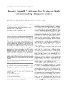
1. Introduction 1.1. Intraguild Predation In many aquatic ecosystems, invertebrate predators such as predatory crustaceans (IG-prey) compete for food with the planktivorous fish (IG-predator), which, at the same time, may also prey on the predatory crustaceans, thereby creating an intraguild predation (IGP) relationship in the system [1–3] (Figure 1). IGP is probably more common in lakes than so far documented [4]. The theory predicts that productivity and the relative efficiency of resource (shared prey) utilization determine the outcome of interactions between IG-predators and IG-prey [2,5].

Biology 2017, 6, 22; doi:10.3390/biology6020022

www.mdpi.com/journal/biology

Biology 2017, 6, 22 Biology 2017, 6, 22

2 of 19 2 of 19

Figure component. F, F, Z1,Z1, Z2,Z2, and P, Figure1.1.Schematic Schematicfood foodweb webininan anaquatic aquaticecosystem ecosystemcontaining containingananIGP IGP component. and are fish,fish, predatory zooplankton, herbivorous zooplankton, and and phytoplankton, respectively. Fz1 and P, are predatory zooplankton, herbivorous zooplankton, phytoplankton, respectively. Fz1 Fz2 ratesrates for Z1 Z1z1Z1z1 and and Z1z2Z1z2 are Z1 ratesrates for andare Fz2the arefish thepredation fish predation forand Z1 Z2, andrespectively. Z2, respectively. arepredation Z1 predation predatory and herbivorous zooplankton, respectively. for predatory and herbivorous zooplankton, respectively.

1.2. Modeling Modeling Intraguild Intraguild Predation Predation 1.2. Tofully fullyunderstand understand an an ecosystem ecosystem that that includes includes IGP IGP dynamics, dynamics, aa separate separate analysis analysis of of the the IGP IGP To components and their impact kind of of analysis cancan be carried out components impact on onthe theecosystem ecosystemisisnecessary. necessary.This This kind analysis be carried using methods in in which the predation out using methods which theabundance, abundance,distribution, distribution,diet, diet, consumption consumption rates, rates, and predation pressureofofthe therelated related IGP components studied [6,7]. However, rigorous long-term empirical pressure IGP components areare studied [6,7]. However, rigorous long-term empirical tests tests of equilibrium IGP interactions are rare [5,8–10], and long-term studies of IGP in natural of equilibrium IGP interactions are rare [5,8–10], and long-term studies of IGP in natural systems are systems are [11,12], even scarcer where conditions are far from and influenced by even scarcer where [11,12], conditions are far from equilibrium andequilibrium influenced by external drivers. external drivers. An alternative explore food web dynamics that include IGPnumerical dynamics An alternative approach to exploreapproach food webto dynamics that include IGP dynamics is by using is by usingmodels. numerical ecosystem models. ecosystem Food webs webs in in which which invertebrate invertebrate predators predators are are important important cannot cannot be be modeled modeled as as aa simple simple chain, Food as is regularly done in aquatic ecosystem models. Adding a compartment for invertebrate predators as is regularly done in aquatic ecosystem models. Adding a compartment for invertebrate predators intolake lakefood foodweb webmodels modelsintroduces introducesan anelement elementof ofIGP IGP[1,2,8]. [1,2,8].ItIt is is also also necessary necessary to to add add an an element element into of cannibalism/self-limitation, cannibalism/self-limitation, ififobserved models areare solved analytically andand are of observedininreality reality[13]. [13].Such Such models solved analytically used to explore ecological issues such as coexistence in IGP systems [14,15], alternative stable states are used to explore ecological issues such as coexistence in IGP systems [14,15], alternative stable [16], and of unstable dynamics, as well as problems in applied ecology suchsuch as the states [16],the andpossibility the possibility of unstable dynamics, as well as problems in applied ecology as biological control of of pest species, the transfer [17], and and the biological control pest species, the transferofofpollutants pollutantsthrough throughthe thepelagic pelagic food food web [17], the conservation conservationof ofthreatened threatenedspecies species[18]. [18]. the Although there there is is much much variability variability among among ecosystems, ecosystems, aa known known result result of of these these models models is is that that Although coexistence is feasible if the IG-prey is better than the IG-predator at competing for the shared prey, coexistence is feasible if the IG-prey is better and ifif the the IG-predator IG-predator accrues accrues aa sufficient sufficient gain gainfrom fromattacking attackingthe theIG-prey IG-prey[1,19]. [1,19]. An An IG-predator IG-predator and that is is superior superior at at suppressing suppressing the the target targetherbivore herbivore population population would would stress stress an an IG-prey IG-preypopulation population that to extinction through a combination of competition and predation [1,19,20]. Additionally, Holt and and to extinction through a combination of competition and predation [1,19,20]. Additionally, Holt Polis[1] [1]showed showedthat thatecosystems ecosystems with IGP have potential to generate alternative Polis with IGP have the the potential to generate alternative stablestable states,states, with with unstable dynamics that to transient However, these are models several unstable dynamics that lead tolead transient phases. phases. However, these models basedare on based severalon arguable arguable assumptions, such (1) the is to assumed to be at equilibrium and the assumptions, such as: (1) theas: system is system assumed be at equilibrium and the models aremodels solvedare to solved to equilibrium withmeteorological constant meteorological or,predators (2) the two predators equilibrium with constant forcing dataforcing [8,21]; data or, (2)[8,21]; the two compete for compete for only a single species of shared prey. Yet, according toand Rosenheim [22], the only a single species of shared prey. Yet, according to Rosenheim Harmonand [22],Harmon the inclusion of inclusionherbivore of multiple prey into IGP the models excludes prediction that the IGP is multiple preyherbivore into IGP models excludes prediction that the the IGP is uniformly disruptive uniformly tothe biological (i.e., the to ability of the IGP-predator to suppress to biologicaldisruptive control (i.e., ability ofcontrol the IGP-predator suppress populations of herbivores); or, populations of herbivores); or, (3) the direct intraguild interactions are sufficiently common to be (3) the direct intraguild interactions are sufficiently common to be important for the IGP dynamics [23]. important formodels the IGP [23]. While simple models canoperating often reproduce thesystems elementary While simple candynamics often reproduce the elementary processes in complex and processes operatingecological in complex systems reveal fundamental ecological [24],able more reveal fundamental patterns [24],and more complex mechanistic food webpatterns models are to complex mechanistic food web models are able to respond to the underlying variability in the physical-chemical conditions over a range of time-scales, and may better describe the natural

Biology 2017, 6, 22

3 of 19

respond to the underlying variability in the physical-chemical conditions over a range of time-scales, and may better describe the natural feeding interactions [25]. A sufficient level of detail in IGP models is therefore essential for developing a deeper understanding of the predation rates and dynamics of zooplankton and fish, and their spatial and temporal variability [26]. However, to date, the explicit implementation and analysis of IGP in freshwater ecosystem models has been surprisingly rare. 1.3. Intraguild Predation in Lake Kinneret The IGP component in the Lake Kinneret food web consists of the dominant fish in the lake, the zooplanktivorous Mirogrex terraesanctae [27], commonly known as Lavnun, and the predatory invertebrates (cyclopoid copepods); both feed on herbivorous zooplankton, while the fish also feed on the cyclopoid copepods. For more than two decades (1970–1993), the Lavnun constituted an important share of the Lake Kinneret commercial fishery, with a fairly constant catch of ~1000 t·y−1 [28]. In the winter of 1991/92, and again in 2002/03, the Lavnun fishery collapsed as the population became devoid of individuals of commercially harvestable sizes (>12 cm, [29]). This was in tandem with exceptionally high precipitation in the winter of 1991/92, and again in 2002/03, leading to >4 m rise in the lake’s water level, with major changes to littoral habitats where the Lavnun spawns. Hydroacoustic surveys indicated that the abundance of mainly sub-commercial sized Lavnun in Lake Kinneret in 1993, and again in 2004, increased by 8–10 fold in comparison to fish abundance levels prior to the flood years [30]. These exceptional increases in fish density were the consequence of the unusually successful recruitment of Lavnun as a result of the extreme water level increases. Hereafter, the term “atypical” will refer to an exceptionally high fish abundance (an abundance which is eight fold or higher than the multiannual average), as was observed approximately one to two years after an atypical high inflow winter. During the 1980s and early 1990s, crustacean (predatory) zooplankton biomass dropped precipitously, reaching its lowest ever annual mean value (0.57 gww ·m−3 ) by 1993, in tandem with the collapse of the Lavnun fishery [31]. Furthermore, the predatory zooplankton underwent a regime shift due to the marked changes in abundance, evident as a gradual replacement of the larger-bodied Mesocyclops sp. with the smaller-bodied Thermocyclops sp. [32]. Gophen et al. [33,34] argued that Lake Kinneret demonstrates a top-down controlled system in which the Lavnun serves as the major predator of herbivorous zooplankton. Based on this assumption, a subsidized dilution program of the Lavnun was initiated as a management policy in 1995 and continued until 2006, whereby an annual amount of 400–500 t of commercial and sub-commercial size Lavnun fish were harvested. The objective of this subsidized harvest was to reduce the predation pressure on zooplankton, leading to an increase in their abundance and a reduction of phytoplankton, through grazing pressure, and ultimately, an improvement of the water quality. However, no correlation was found between the subsidized harvest and the Kinneret Water Quality Index [35] or other water quality indicators, suggesting that top-down control was not occurring as hypothesized. Blumenshine and Hambright [6] compared the potential predation pressure on Lake Kinneret herbivorous zooplankton by Lavnun with that of the cyclopoid copepods. Despite having a much lower biomass than Lavnun, cyclopoid copepods accounted for a greater portion of the predation mortality of herbivorous zooplankton. This suggested that the intentional removal of Lavnun would not result in a subsequent increase in herbivorous zooplankton biomass as expected according to top-down theory. Instead, a reduction in Lavnun predation pressure may allow for an increase in the abundance of cyclopoid copepod and thereby result in a net increase in the predation pressure on herbivorous zooplankton. A food web model developed for Lake Kinneret by Hart et al. [36] also predicted that planktivorous fish may serve as minor predators of herbivorous zooplankton, with the majority of its top-down regulation associated with cyclopoid copepods. Hart [13] explored the effects of IGP and self-limiting factors on the top-down and bottom-up properties of Lake Kinneret using the different models constructed based on the Lake Kinneret carbon flux model. The results indicated that IGP can reduce or even reverse the top-down effects predicted by the food chain theory, as a decrease

Biology 2017, 6, 22

4 of 19

in planktivorous fish is accompanied by an increase in the predation of zooplankton on invertebrates, and that the degree of self-limitation among the IG-prey is a key factor in determining the direction and strength of the top-down response. Although models such as Hart et al. [36] and Hart [13] extended our understanding of ecosystems that have an IGP component, they are limited in their ability to reveal insights into the details of IGP variability. In particular, we are interested in understanding how these IGP-dynamics respond to a highly variable physico-chemical environment and the associated complex patterns of planktonic succession [36–41]. Moreover, Roelke et al. [42] analyzed a long-term data-set of Lake Kinneret within the framework of an alternative states model and revealed a possible complex triggering mechanism and system hysteresis (e.g., a change in a variable threshold where alternative states are possible, to a threshold where alternative states will no longer be possible). Gal and Anderson [32] identified the occurrence of a regime shift in the zooplankton population. Therefore, to explore the IGP relationship under the non-equilibrium conditions of Lake Kinneret, we applied a complex aquatic ecosystem model (DYCD-FISH). Unlike the models of Hart [13], that capture the most important first-order interactions by means of simple physics, DYCD-FISH is able to simulate the seasonal dynamics of vertical stratification and the most important chemical and biological ecosystem components. DYCD-FISH has previously been configured to include the IGP trophic triangle [43], accounting for both the bottom-up and top-down pathways shaping the seasonal dynamics of biogeochemical and ecological processes. However the intricacies of the IGP relationship, as described above, were not considered. The aims of this study were therefore: (1) to improve our understanding of the predator-prey interactions between the dominant fish species in Lake Kinneret, Mirogrex terraesanctae, and zooplankton; (2) to study the sensitivity of the key factors controlling the IGP triangle (e.g., predation rate, feeding preference, and vulnerability to fish predation); (3) to compare IGP dynamics during “atypical” conditions, whereby an extreme increase in the fish population occurs, relative to “typical” conditions; and (4) to explore the likely impacts of fishery biomanipulation on fish and zooplankton biomass. 2. Materials and Methods DYCD-FISH was validated for Lake Kinneret as previously described in Gal et al. [39] and Makler-Pick et al. [43]. The model is briefly described below. 2.1. Ecological Configuration The mechanistic model DYCD-FISH was used to simulate the interactions between the hydrodynamics, biogeochemistry, bacteria, phytoplankton, zooplankton, and fish within Lake Kinneret. DYRESM-CAEDYM (DYnamic REservoir Simulation Model-Computational Aquatic Ecosystem DYnamics Model, DYCD) is a one-dimensional coupled hydrodynamic-ecological model. DYRESM predicts the vertical distribution of temperature, salinity, and density, and models surface heat, mass and momentum transfers, mixed layer dynamics, hypolimnetic mixing, benthic boundary layer mixing, inflows, and outflows [44]. The model represents the lake as a series of homogeneous horizontal Lagrangian layers of variable thickness that expand or contract according to the degree of stratification and mixing, and the inflows or outflows entering or leaving the lake. CAEDYM is a generic aquatic ecological model in which a series of ordinary differential equations are solved to describe changes in the concentrations of nutrients (C, N, P, Si), detritus, dissolved oxygen, phytoplankton, and zooplankton, as a function of environmental forcing and ecological interactions for each layer represented by DYRESM. The variables of irradiance, temperature, salinity, and density are passed to CAEDYM, typically at a 1-h time step, and are used to determine the rates of change of biomass and chemical constituents for each of the ecological state variables. DYCD-FISH couples a fish population model with DYCD to create a combined ecosystem-fish model capable of integrating the relatively slow metabolism of fish with other ecosystem components

Biology 2017, 6, 22

5 of 19

that often respond faster than fish. The model also accounts for the direct and indirect feedback between fish dynamics and the biogeochemical and planktonic modules. Fish directly affect the concentrations of the zooplankton, the particulate and dissolved organic matter (POM and DOM, respectively), oxygen, and the dissolved inorganic carbon in the different layers where the fish are located. Specifically, the Lake Kinneret version of DYCD-FISH is configured to simulate the carbon, nitrogen, phosphorus, and oxygen cycles, along with the biomass and metabolic processes of five phytoplankton groups (the dinoflagellate Peridinium gatunense; the filamentous diatom Aulacoseira granulata; the toxin-producing, N-fixing filamentous cyanobacterium Aphanizomenon sp.; the toxic colonial cyanobacterium that does not fix gaseous N, Microcystis sp.; and a general group of small-cell species, termed nanoplankton), three zooplankton groups (predatory zooplankton: adult stages of the predatory copepods and predatory rotifers; herbivorous zooplankton: cladocerans and copepodites; and micro-zooplankton including flagellates, ciliates, and copepod nauplii), heterotrophic bacteria (all simulated in units of mgC·L−1 ), and the population dynamics of the dominant fish in Lake Kinneret, Mirogrex terraesanctae [27]. The fish sub-model is based on a generic bioenergetics formulation, whereby an energy balance equation equates the energy gained as the difference between that consumed and metabolic expenses. Specifically, energy gain occurs through the difference between consumption and respiration, excretion, egestion, specific activity, and reproduction. The energy gained affects the growth rate and fish wet weight, and therefore, the growth rate of an individual fish is represented as the daily changes in wet weight per unit of fish weight per day (gww ·gfish −1 ·day−1 ). In DYCD-FISH, the bioenergetics model is applied to many “super-individuals”, where each “super individual” represents numerous similar individuals [45], which each experience processes such as recruitment, and natural and fishing mortality that dynamically affect the number and biomass of fish. The population model takes advantage of the 1D hydrodynamic model, and at each time step, based on ambient conditions, the fish are redistributed in the water column with some stochastic variability, imitating the natural spatial movement and spread of the fish. Since the model is spatially (vertically) explicit, zooplankton, phytoplankton, and fish are located in varying water layers, such that the feeding intensity depends on the habitat overlap between predator and prey. Additionally, an explicit recruitment model was developed to simulate the reported linkage between the change in water level and Lavnun spawning success. The specific parameters and customization used in the current fish population model are described in Makler-Pick et al. [43]. The fish-related variables examined in this study included fish biomass and the fish predation rate for zooplankton. Since the focus of the manuscript is on fish-related food web dynamics associated with the IGP, we will now describe relevant components and interactions included in the Lake Kinneret implementation of DYCD-FISH. The Lavnun (the IG-predator) is an endemic, visually orienting zooplanktivore. As evident by the positive electivity values (i.e., preferences to food source) for Cladocera and Copepoda [46], it mainly feeds on Cladocera and Copepoda. The diet composition of the Lavnun also includes micro-zooplankton and particulate detrital material. When there are multiple prey types, the actual consumption depends on prey densities, the vulnerability of each prey item to the predator, the half-saturation constants governing the rate of feeding, and the maximum daily ration at a particular mass and temperature. Prey vulnerability, defined in the literature as the product of the encounter rate between predator and prey and the capture success of the predator [47], is dependent on several factors, such as abiotic conditions, the relative size of predator and prey, and predator activity and movements. Here, however, because of the lack of vulnerability experimental data, we used stomach content analysis [48,49] as an indicator of prey vulnerability and set the initial food vulnerability of the predatory zooplankton, herbivorous zooplankton, and micro-zooplankton to fish predation rates of 0.4, 0.5, and 0.02, respectively. The advantage of the current model is that it enables an exploration of the theoretical impacts of imprecise parameters, such as food vulnerability, the predation rate, and feeding preference, by substantially modifying their values. The diet of the

Biology 2017, 6, 22

6 of 19

predatory zooplankton, the IG-prey, consists of micro-zooplankton, herbivorous zooplankton, and the early stages of predatory zooplankton (via self-limiting predation) with preferences of 0.5, 0.35, 0.15, respectively. The main dietary source of herbivorous zooplankton (the IGP basal resource) is a multi-species group of small-celled phytoplankton termed the nanoplankton. 2.2. Model Base-Case Simulations The simulations were configured to run from Jan. 1997 to Sep. 2003, at a 1 h time step for DYCD and a daily time step for the fish model. The initial conditions, forcing data, and input data are as described in Gal et al. [39] and Makler-Pick et al. [43]. The initial number of fish was set to 100 million fish in the lake (hereafter, ×1 or base level), as validated in Makler-Pick et al. [43]. The model time-series output files were used to study the temporal dynamics of zooplankton and fish biomass, as well as the predation rates of both fish and predatory zooplankton (the model is available upon request from the software developers). Multiple simulation runs verified that the stochastic component within the individual-based fish model resulted in negligible differences in fish population behavior for repeated simulation runs. 2.3. IGP Scenarios and Sensitivity Analysis To simulate IGP dynamics when the number of fish is higher than the multiannual average, a series of scenarios were conducted, in which the number of fish represented by each “representative” super-individual was changed. The lake-wide fish population was initialized with 1000 “representative” fish, each set to represent 100,000 fish in the lake, equating to 100,000,000 fish in total. Then, this number was changed from an initial number of 100,000 (×1) to 200,000 (×2), and then up to 800,000 (×8) fish per “representative” fish, which was higher than the estimated increase in fish density recorded in 2004 [30], but enabled us to examine an extreme situation. Based on the outcome of the scenarios, we studied the impact of increasing fish numbers on the zooplankton biomass and predation rates. The results of complex models often suffer from limitations due to various sources of error and uncertainty, such as the initial conditions, input data, model structure, model parameters, and validation data [50]. However, a large source of model uncertainty is associated with the parameter values [50,51]. When a high uncertainty in the value of a parameter coincides with a high sensitivity of the model to that parameter, the reliability of the model predictions may be very low [52]. Makler et al. [53] and Gal et al. [54] evaluated the sensitivity of DYCD model parameters. Here, the sensitivity of the herbivorous zooplankton to different key factors playing a part in the IGP triangle are explicitly studied. The initial values of the following parameters: the maximum predation rate of the predatory zooplankton (gmax , gC·m−3 (gZ·m−3 )−1 ·day−1 ), the feeding preference of predatory zooplankton to the early stages of predatory zooplankton (cannibalism or self-limiting predation) (Pzk1 ), and the vulnerability of predatory (V11 ) and herbivorous (V12 ) zooplankton to fish predation, were modified. The changes were made over the course of a series of scenarios by changing the initial value of each parameter, one at a time, by ±50%. The average concentration of the herbivorous zooplankton over the seven-year simulation was calculated and served as the basis for comparison. 2.4. Biomanipulation Fish biomanipulation (namely, the positive size-selective harvest of mainly non-commercial size fish) is a possible management action aiming to control high fish recruitment, such as occurs in Lake Kinneret in atypical years, to reduce phytoplankton and ultimately improve the water quality. The size-selective harvest of the Lavnun was modeled by increasing the value of the fishing mortality (exploitation rate) parameter of non-commercial size fish from 0 to 50 (%·year−1 ), and the value of the fishing mortality parameter of commercial size fish from 28 to 50 (%·year−1 ), based on the scenario of an atypical year (×8 scenario).

Biology 2017, 6, 22 Biology 2017, 6, 22

7 of 19 7 of 19

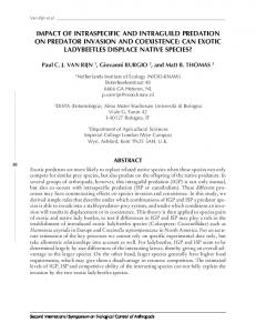
3. Results 3.1. IGP Dynamics Dynamics under 3.1. IGP under Typical Typical Conditions Conditions The ×1) showed showed seasonal seasonal biomass The herbivorous herbivorous zooplankton zooplankton in in the the base base simulation simulation level level((×1) biomass peaks peaks from fall to spring, with low inter-annual variation throughout the simulation period (Figure 2A). 2A). from fall to spring, with low inter-annual variation throughout the simulation period (Figure The predatory zooplankton (cyclopoid copepods) showed annual biomass peaks in late winter to early The predatory zooplankton (cyclopoid copepods) showed annual biomass peaks in late winter to spring, with low valuesvalues (Figure 2B). 2B). early spring, withinterim low interim (Figure

Figure 2. Simulation results (1/1/1997–1/9/2003) of (A) herbivorous zooplankton concentration Figure 2. Simulation results (1/1/1997–1/9/2003) of (A) herbivorous zooplankton concentration (mgC·L−1) and (B) predatory zooplankton concentration (mgC·L−1) at base level of fish (×1). (mgC·L−1 ) and (B) predatory zooplankton concentration (mgC·L−1 ) at base level of fish (×1).

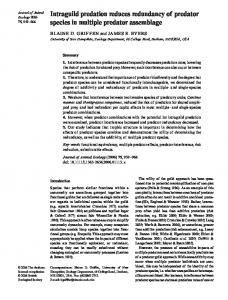
The average simulated lake-wide total biomass of predatory cyclopoid over the years 1997– The simulated lake-wide biomass of predatory cyclopoid over years 1997–2003, 6 gww, with −1. During 2003, wasaverage 799 × 10 a meantotal daily predation rate of 109 mgprey· gpred−1the ·day this 6g −1 ·day−1 . During this period, was 799 × 10 , with a mean daily predation rate of 109 mg · g ww prey 6 pred period, the Lavnun had an average total lake biomass of 1281 × 10 gww and the mean daily predation the Lavnun had an average total lakewas biomass 106−1g. ww the mean daily predation −1·day pressure on herbivorous zooplankton 28 mgofprey1281 ·gpred× Theand simulated predation pressure − 1 − 1 pressure on herbivorous zooplankton was 28 mg · g · day . The simulated predation pressure prey pred by both the Lavnun and the predatory zooplankton varied seasonally. During winter and early by both the Lavnun and the predatory zooplankton varied seasonally. During winter and early spring (November-February), predation by predatory zooplankton accounted for the majorityspring of the (November-February), by predatory zooplankton accounted for the majority of the predation predation mortality forpredation herbivorous zooplankton (Figure 3A), imposing a predation pressure 10–20 mortality for herbivorous zooplankton (Figure 3A),(Figure imposing times higher than the Lavnun predation pressure 3B).a predation pressure 10–20 times higher than At thethe Lavnun pressure 3B). the monthly average predation rate of predatory time predation of its annual peak, (Figure in December, At the time its annual December, the monthly average predation predatory zooplankton wasof 7.0 μgC·L−1peak, ·day−1in(10% of herbivorous zooplankton biomassrate perof day), and −1 ·day−1 (10% of herbivorous zooplankton biomass per day), and remained zooplankton was 7.0 µgC · L −1 −1 remained high in January, before declining to very low levels (0.004 μgC·L ·day ) between March 1 ·day−1 ) between March and October high January, before 4A). declining to very levels (0.004the µgC ·L−predation and in October (Figure During thislow time period, fish rate was higher than the (Figure 4A). During this time period, the fish predation rate was higher than the zooplankton predation zooplankton predation rate (Figure 4B). The annual cycle of the fish predation rate was more rate (Figure 4B). The annual cycle of the fish predation rate was more moderate than that of the predatory moderate than that of the predatory zooplankton, ranging between a minimum of 0.2 μgC·L−1·day−1 zooplankton, between of a minimum 0.2−1µgC ·L−1 ·day−1 (1% in September, to a maximum of in September,ranging to a maximum 0.7 μgC·L−1of·day in November of herbivorous zooplankton − 1 − 1 0.7 µgC·Lconcentration ·day in November biomass per day). (1% of herbivorous zooplankton biomass concentration per day).

Biology Biology 2017, 2017, 6, 6, 22 22 Biology 2017, 6, 22

88 of of 19 19 8 of 19

−1) of predatory zooplankton (thin line) and fish Figure 3. (A) Simulated predation rate (μgC·L−1−1−·day 1 ·day 1 of predatory zooplankton (thin line) and −1) − Figure 3. (A) (A) Simulated Simulated predation predationrate rate(μgC·L (µgC·L ·day of)predatory zooplankton (thin line) and fish (thick line) on herbivorous zooplankton; (B) Ratio of the zooplankton predation rate (Z1z2) to the fish (thick line) on herbivorous zooplankton; (B) Ratio of the zooplankton predation rate rate (Z1z2 (thick line) on herbivorous zooplankton; (B) Ratio of the zooplankton predation z2)) to the fish-predation rate (Fz2) for herbivorous zooplankton (Z2) at the base level of fish (thin line) and at an fish-predation rate (F ) for herbivorous zooplankton (Z2) at the base level of fish (thin line) and at z2) for herbivorous zooplankton (Z2) at the base level of fish (thin line) and fish-predation rate (Fz2 at an increased level of fish (×8, thick line). an increased level of fish 8, thick line). increased level of fish (×8,(×thick line).

Figure 4. Simulated monthly average predation rate (μgC·L−1·day−1) of (A) predatory zooplankton and (B) fish, on herbivorous zooplankton (Z2) at base fish level (×1). −1 day−1) of (A) predatory zooplankton Figure 4. 4. Simulated Simulatedmonthly monthlyaverage averagepredation predationrate rate(µgC (μgC·L −1 ) of (A) predatory zooplankton Figure ·L−1 ··day and (B) fish, on herbivorous zooplankton (Z2) at base fish level (×1). and (B) fish, on herbivorous zooplankton (Z2) at base fish level (×1).

Biology 2017, 6, 22 Biology 2017, 6, 22

9 of 19 9 of 19

From fish predation predationwas wasthe thedominant dominantloss lossofofherbivorous herbivorous zooplankton, From spring spring to autumn, fish zooplankton, in in tandem with a 40% lower herbivorous zooplankton biomass in comparison to late winter tandem with a 40% lower herbivorous zooplankton biomass in comparison late winter (November–February, and 5). However, in lateinwinter, during the short period of the (November–February, Figures Figure 52A and Figure 2A). However, late winter, during the short period of annual biomass peak of the of predatory zooplankton, there was an extremely high predation mortality the annual biomass peak the predatory zooplankton, there was an extremely high predation (>80% of total herbivorous zooplankton) associated associated with zooplankton predation. predation. mortality (>80% of total herbivorous zooplankton) with zooplankton

Figure5.5.Simulated Simulatedproportion proportion(%) (%)of oftotal totalherbivorous herbivorouszooplankton zooplanktonmortality mortalitydue dueto tonon-predation non-predation Figure mortality (light grey), zooplankton-predation (black), and fish-predation (dark grey). mortality (light grey), zooplankton-predation (black), and fish-predation (dark grey).

3.2. IGP IGP Dynamics Dynamicsduring duringHigh HighFish FishAbundance Abundance 3.2. Throughout most most of ofthe thehigh highfish fishabundance abundancesimulation simulation(× (×8), the concentration concentration of of predatory predatory Throughout 8), the zooplankton and micro-zooplankton was lower than in the base level scenario (ratio < 1 in Figure 6A zooplankton and micro-zooplankton was lower than in the base level scenario (ratio < 1 in Figure 6A,C). andherbivorous 6C). The herbivorous zooplankton biomass was also affected by the changes in fish densities. The zooplankton biomass was also affected by the changes in fish densities. This impact, This impact, however, mainly occurred in the periods between the seasonal biomass peaks of the however, mainly occurred in the periods between the seasonal biomass peaks of the herbivorous herbivorous zooplankton. In of thehigher presence higher fish the concentration herbivorous zooplankton. In the presence fish of numbers, the numbers, concentration of herbivorousofzooplankton zooplankton during its simulated seasonal biomass peaks (January–February) was similar or even during its simulated seasonal biomass peaks (January–February) was similar or even higher than the higher than the concentration simulated at the base level of fish. This phenomenon is indicated by concentration simulated at the base level of fish. This phenomenon is indicated by values higher than values higher6B. than one in Figure 6B. one in Figure In the presence of ××8 more fish, fish, fish fish predation predation of of herbivorous herbivorous zooplankton zooplankton dominates dominates the the In the presence of 8 more predation in this group for most of the simulation period (values < 1 in Figure 3B), with some predation in this group for most of the simulation period (values < 1 in Figure 3B), with some exceptionsduring during fourth, and seventh of the simulation, when the ratio of exceptions thethe fourth, sixth,sixth, and seventh year of year the simulation, when the ratio of zooplankton zooplankton predation to fish predation was greater than one. predation to fish predation was greater than one. Substantialdifferences differences between the zooplankton pressure on zooplankton herbivorous Substantial between the zooplankton predationpredation pressure on herbivorous zooplankton in the ×8 scenario and the ×1 simulation are mainly observed during the annual of in the ×8 scenario and the ×1 simulation are mainly observed during the annual peak peak of the the herbivorous zooplankton biomass, demonstrating a considerable seasonal decrease in the net herbivorous zooplankton biomass, demonstrating a considerable seasonal decrease in the net predation predation by predatory-zooplankton at the ×8(Figure scenario 7). Intriguingly, lower predation by predatory-zooplankton at the ×8 scenario 7).(Figure Intriguingly, the lower the predation pressure pressure may allow for an increase in herbivorous zooplankton biomass during these may allow for an increase in herbivorous zooplankton biomass during these periods (Figure 6B).periods At all (Figure 6B).model At all other times, suggest model simulations suggest that the herbivorous biomass other times, simulations that the herbivorous zooplankton biomasszooplankton is mainly controlled is mainly controlled by fish predation. by fish predation.

Biology 2017, 6, 22 Biology 2017, 6, 22 Biology 2017, 6, 22

10 of 19 10 of 19 10 of 19

Figure 6. Ratio of zooplankton concentration at ×8 to zooplankton concentration at ×1 for (A) Figure 6. 6.Ratio concentrationatat×8×to 8 to zooplankton concentration ×1(A)for Figure Ratio of of zooplankton zooplankton concentration zooplankton concentration at ×1atfor predatory zooplankton, (B) herbivorous zooplankton and (C) micro zooplankton. (A)predatory predatoryzooplankton, zooplankton,(B) (B) herbivorous zooplankton and (C) micro zooplankton. herbivorous zooplankton and (C) micro zooplankton.

Figure 7. The difference between the predatory zooplankton (Z1) predation rate (on herbivorous Figure The difference Figure 7. 7. The difference between between the the predatory predatory zooplankton zooplankton (Z1) (Z1) predation predation rate rate (on (on herbivorous herbivorous zooplankton, Z2) at the base simulation (×1) and the ×8 scenario. Values represent the whole lake zooplankton, simulation ( × 1) and the × 8 scenario. Values represent the whole zooplankton, Z2) Z2) at at the the base base simulation (×1) and the ×8 scenario. Values represent the whole lake lake −1 predation rates in ton day −1 . predation predation rates rates in in ton ton day day−1. .

The mean annual predation by fish and zooplankton on the different zooplankton groups at The by are fishgiven and zooplankton thebase different zooplankton varyingmean levelsannual of fishpredation abundance, in Table 1. Atonthe level (×1), the meangroups annual at varying levels of fish abundance, are given in Table 1. At the base level (×1), the mean annual predation of predatory zooplankton is 2.5, 5.3, and 7.7 times higher than fish predation on predation of predatory zooplankton is 2.5, 5.3, and 7.7 times higher than fish predation on

Biology 2017, 6, 22

11 of 19

The mean annual predation by fish and zooplankton on the different zooplankton groups at varying levels of fish abundance, are given in Table 1. At the base level (×1), the mean annual predation of predatory zooplankton is 2.5, 5.3, and 7.7 times higher than fish predation on herbivorous, predatory, and micro-zooplankton, respectively. These results demonstrate the predation superiority of the predatory zooplankton (over the fish) at the base level of fish. An increase in the number of fish resulted in a lower mean annual predation rate of predatory zooplankton, both on itself (i.e., self-limitation) and on the other zooplankton groups. The main impact was on the predatory zooplankton itself; the self-limitation was lowered to 9% of the base level in the presence of ×8 more fish. On average, the outcome of the ×8 scenario was a 70% lower total zooplankton predation (on all zooplankton groups), and on the other hand, a higher fish predation, on all its prey types (>200%). Interestingly, the total herbivorous zooplankton eaten annually, whether by fish or by zooplankton, was close to 44 × 103 ton year−1 for all simulated scenarios, regardless of fish biomass. The total predation in the system (the sum of zooplankton predation and fish predation) ranged from 52 × 103 to 60 × 103 ton. At the base level of fish, and even when the number of fish was doubled, the ratio between the annual average of zooplankton predation to the annual average of fish predation on all zooplankton groups was greater than one, indicating that, in total, the main predator in the ecosystem is the predatory zooplankton (Table 1). A higher number of fish (×8) resulted in a ratio lower than one, indicating the dominance of fish in consuming zooplankton under these conditions. Table 1. Comparison of the fish (F) and zooplankton (Z) average annual predation rate (thousand ton year−1 ) and ratio of zooplankton predation to fish predation for each zooplankton group, at base level of fish (×1), at ×2 fish, and at ×8 fish. Values in parentheses indicate the relative fraction (in %) of predation pressure compared to the base level. Z1z1 , Z1z2 , and Z1z3 are predatory zooplankton predation on predatory (Z1), herbivorous (Z2), and micro (Z3) zooplankton, respectively. Fz1 , Fz2 , and Fz3 are fish predation on predatory, herbivore, and micro zooplankton, respectively. Variable

×1

×2

×8

Z1z1 Fz1 Z1z2 Fz2 Z1z3 Fz3 Total Zzi predation Total Fzi predation Total predation Total predation on Z2 (Z1z2 + Fz2 ) Z1z1 /Fz1 Z1z2 /Fz2 Z1z3 /Fz3

12.62 2.37 31.81 12.83 0.59 0.08 45.02 15.28 60.3 44.64 5.32 2.48 7.7

6.89 (54%) 3.48 (146%) 25.32 (79%) 18.57 (144%) 0.45 (75%) 0.13 (162%) 32.66 (76%) 22.19 (145%) 54.84 43.89 1.98 1.36 3.4

1.17 (9%) 5.01 (211%) 12.11 (38%) 33.10 (258%) 0.16 (27%) 0.35 (438%) 13.43 (30%) 38.45 (252%) 51.9 45.21 0.23 0.37 0.45

3.3. The Effect of Biomanipulation Manipulating the fishery by imposing particularly heavy fishing mortality on non-commercial (