This links Gage, Hamilton and Grayson`s result of the curvature. 1We use subscript g to denote ..... 7] M Gage and R S Hamilton. The heat equation shrinking ...
Intrinsic Scale Space for Images on Surfaces: The Geodesic Curvature Flow Ron Kimmel�
Lawrence Berkeley National Laboratory, and Dept. of of Mathematics, Univ. of California, Berkeley, CA 94720. Abstract A scale space for images painted on surfaces is introduced. Based on the geodesic curvature ow of the iso-gray level contours of an image painted on the given surface, the image is evolved and forms the natural geometric scale space. Its geometrical properties are discussed as well as the intrinsic nature of the proposed ow. I.e. the
ow is invariant to the bending of the surface.
1 Introduction In this note we introduce and study a geometric scale space for images painted on a given surface. We show that a natural scale for images painted on surfaces can be constructed by considering the iso-gray levels of the image as curves on the surface, and nding the proper geometric heat ow in the metric induced by the immersion. Speci cally, we study the properties of the geodesic curvature scale space (� scale space) for images that are painted on a given surface. Recently, surface curves ow by their geodesic curvature was studied in [9], numerically implemented for curves with and without xed end points in [12, 3], and used for re nement of initial curves into geodesics (shortest paths on surfaces) in [11]. In [9] Grayson studies the evolution of smooth curves immersed in Riemannian surfaces according to their geodesic curvature ow (� ow). The � ow is often called curve shortening ow since the ow lines in the space of closed curves are tangent to the gradient of the length functional. It is the fastest way to shrink curves using only local (geometrical) information. The curvature ow is also referred to as the Heat Flow on Isometric Immersion since it is the heat equation as long as the heat operator is computed in the metric induced by the immersion. Grayson showed that as curves evolve according to the geodesic curvature ow, the embedding property is preserved, and the evolving curve exists for all times and either becomes g
g
g
This work is supported in part by the Applied Mathematics Subprogram of the O�ce of Energy Research under DE-AC03-76SFOOO98, and ONR grant under NOOO14-96-1-0381. �
1
a geodesic or shrinks into a point. We will limit our discussion to smooth Riemannian surfaces which are convex at in nity (the convex hull of every compact subset is compact). Moreover, we shall deal only with surfaces which are given as a parameterized function in a bounded domain. Given these conditions, one can apply Grayson`s Theorem 0.1 in [9] that states that the � ow shrinks closed curves to points while embedding is preserved. Open curves` behavior depends on the boundary conditions, and could either disappear at a point in nite time or converge to a geodesic in the C 1 norm, i.e. the geodesic curvature converges to zero. By open curves we refer to curves that connect two points on the boundary of our nite domain (two points on the image boundaries). We use the equations developed for curves in [12], generalize them, and formulate the natural scale space for images painted on surfaces. This generalization is based on the observation that any gray level image can be expressed as a set of curves that correspond to its iso-gray level curves. Thus, evolving each of these curves according to the � ow leads to the evolution of the whole image, and the construction of the � scale space. Since the � ow is intrinsic, so is the image ow. Given a surface and an image that is painted on that surface, the � ow will be invariant to bending (isometric mapping) of the surface. A simple example is an image painted on a plane. In this planar case, the � ow is equivalent to the planar curvature ow. It was proven in [7, 8] to shrink any planar curve into a convex one and then into a circular point, while embedding is preserved. Assuming that the plane with the image painted on it is bent into a cylinder, applying the � ow on the new image obtained by taking a picture of the cylinder, guarantees that the sequence of evolved images on the surface can be mapped into the sequence of the evolved images on the plane. This mapping is the same one that mapped the initial planar image onto the cylinder. The result is a ow which is invariant to the bending of the surface. g
g
g
g
g
g
g
2 Relation to Existing Scale Spaces Exploring the whole theory and history of scale space and its various applications in image processing and computer vision is beyond the scope of this paper. We refer to [16], for a recent collection of papers dealing with linear and non linear scale spaces. Originally, the classical heat equation I = �I (where �I � I + I ) was considered to be a good candidate for the description of scale . Its linear properties lead to e�cient implementations that could be realized in the Fourier domain with low computational e�ort. The observation that the complexity of the image topology can increase when applying the heat equation (local maximum points can be formed) as well as the need for invariant ows under di�erent transformation groups, lead to the consideration of other, non linear, scale spaces [2, 1, 17]. Most of these non linear ows have a simple and natural mathematical relation to the evolution of the gray level sets of the image. The obvious reason is the requirement for preserving the embedding of the gray level sets along the evolution, as well as the smoothing of the level sets with the scale parameter, so that the topology of the image is simpli ed along the scale. This links Gage, Hamilton and Grayson`s result of the curvature t
xx
yy
1
We use subscript g to denote relation to the metric, like the geodesic curvature �g , and subscripts x; y and t to denote partial derivatives with respect to x; y and t, e.g. Ixx � @ 2 I=@x2. 1
2
ow of planar curves to Gabors' historical image enhancement algorithm [6, 14]. We shall use this natural link between level sets and the image evolution, and the nice properties of the geodesic curvature ow of curves on surfaces, to construct the natural ow for images on surfaces. In [5] the second di�erential operator of Beltrami is considered as a possible operator for the general heat equation under a given xed metric g, namely I = � I . In [19, 13] a new scale space for images in which the image is considered as a surface was introduced, i.e. the metric g is the induced metric (the metric of the image surface). It was shown to give promising results as a selective smoothing operator in color, movies and texture. In that case � I is the projection of the mean curvature vector onto the intensity coordinate. When setting the metric to the identity g = � , � I boils down to the classical heat equation for the 2D case. The relation between the � ow and the � ow, is analog to the relation between the classical heat equation: I = �I , and the 2D geometrical heat equation: I = (I I ? 2I I I + I I )=(I + I ), i.e. the planar curvature (�) ow. This is a natural analogy since considering a plane as the underlying surface, � becomes the Laplacian operator �, and � becomes the planar curvature �. Although the geometric heat equation (� ow) was explored and used for several applications, to the best of our knowledge, the geodesic curvature ow as a scale space has not yet been explored nor any other bending invariant ows. t
g
g
ij
ij
g
g
g
t
t
xx
2
x
y
y
xy
yy
2
2
2
x
x
y
g
g
3 The Geodesic Curvature �g
Let the surface S = (x; y; z(x; y)) be de ned as a parameterized function. Next, consider the surface curve C (s) = (x(s); y(s); z(x(s); y(s))) where s is the arclength parameter of the curve: jC j = 1. The geodesic curvature vector � N^ is de ned as: � N^ = C ? hC ; N iN; where C (the curvature vector) is the second derivative of the curve according to s, and N is the normal to the surface, see Fig. 1. A geodesic curve is a curve along which the geodesic curvature is equal to zero. Thus, any small perturbation of a geodesic curve increases its length. Geodesics are locally the shortest paths on a given surface, and in case there exists a straight line on a surfaces it is obviously a geodesic curve. Evolving a curve on the surface by its geodesic curvature vector eld is the fastest way to shrink the curves` length and thereby evolve it into a geodesic. Another important geometrical property is the invariance of the geodesic curvature to bending of the surface. We will use these two properties, as well as the nice characteristics of this ow that were shown by Grayson [9], to construct the � scale space. s
g
g
ss
ss
ss
g
4 From Curve to Image Evolution on a Surface
Our input is an image I (x; y) that is painted on the given surface S = (x; y; z(x; y)), see Fig. 2. Using the fact the embedding is preserved under geodesic curvature ow of curves on surfaces, we may consider the image as an implicit representation of its iso-gray levels. This 3
N T ^ kgN
C(s) S= (x,y,z(x,y))
C ss
Figure 1: The geometry of the geodesic curvature vector, � N^ . g
is just a mental exercise that will help us derive the geodesic curvature evolution of the image I (x; y) as a function of its rst and second derivatives, as well as the surface derivatives. Let t be the scale variable. Then the main result of this paper is the following intrinsic evolution for I (x; y) given as initial condition to: @I = K (I ; I ; I ; I ; I ; z ; z ; z ; z ; z ); @t where K is the geodesic curvature scale space function. g
x
y
xx
xy
yy
x
y
xx
xy
yy
g
S= (x,y,z(x,y)) z y x
I(x,y)
Figure 2: The image I (x; y) is painted on the parameterized surface S = (x; y; z(x; y)). I.e. the surface point (x; y; z(x; y)) has the gray level I (x; y). The � scale space has the following properties: 1. Intrinsic: Invariant to bending of the surface. 2. Embedding: The embedding property of the level sets of the evolving gray level image is preserved. g
4
3. Existence: The level sets exist for all the evolution time, and disappear at a point in most cases, or converge into a geodesic connecting the boundaries in special cases. 4. Causality: The total geodesic curvature of the level sets is a decreasing function. This is an important property, since combined with the embedding property, it means that the topology of the image is simpli ed along the evolution. 5. Shortening ow: The scale space is a shortening ow of the level sets of the image painted on the surface.
5
�g
Scale Space Derivation
As a rst step we follow [12] and analyze the single curve case of evolution under the �
ow. Then, based on the fact that embedding is preserved, we generalize and consider the whole image. Let C~(~s) = (x(~s); y(~s)) be an iso-gray level planar curve parameterized by its arclength s~ of the image I (x; y). I.e. I (x; y) is constant along C~(~s): I (C~(~s)) = Const; g
or equivalently @I (C~(~s))=@s~ = 0. The iso-gray level curve C~(~s) is the projection onto the (image) coordinate plane of the 3D surface curve C (~s) = (x(~s); y(~s); z(x(~s); y(~s))). I.e. C~(~s) = � � C (~s), where � is the projection operation (a; b) = � � (a; b; c). See Fig. 3. T ^ k gN
C(s) S= (x,y,z(x,y)) z y x
~~ C(s) ~ N
Figure 3: The geometry of the geodesic curvature vector projection. Let us rst show a simple connection between an image and its level sets evolution. Lemma 1 Let C~(~s) = (x(~s); y(~s)) be the level curve of I (x; y). Assume that the planar curve C~ is evolving in the coordinate plane according to the smooth velocity eld V : C~ = V : t
5
Then the image follow the evolution
I = hV ; rI i; where rI � (I ; I ). Proof. The ow C~ = V was shown in [4] to be geometrically equivalent to the normal ~ N~ ; where N~ is the unit normal of the planar curve. By the direction evolution C~ = hV ; Ni chain rule we have @I = @I @x + @I @y @t @x @t @y @t ~ = hr D I; C i E ~ N~ : = rI; hV ; Ni Recalling that C~ is a level set of I (x; y), we can express the normal N~ as N~ = rI=jrI j. Using this relation E @I = DrI; hV ; Ni ~ N~ @t * + r I r I = rI; hV ; jrI j i jrI j = hV ; rI i � jr1I j � hrI; rI i = hV ; rI i: t
x
y
t
t
t
2
Let us now derive the geodesic curvature scale space equation Lemma 2 The geodesic curvature scale space for the image I (x; y) painted on the parameterized surface S = (x; y; z(x; y)) is given by the evolution equation
@I = I I ? 2I I I + I I + x x x2 y y2y (z I ? 2I I z + z I ) : (1) @t I (1 + z ) + I (1 + z ) ? 2z z I I Proof. We start from the evolution of the 3D level sets of I (x; y) on the surface S = (x; y; z(x; y)) that is given by the geodesic curvature ow @C = � N^ : @t Where � N^ is the 3D geodesic curvature vector de ned by � N^ = �N ? h�N ; N iN = C ? hC ; N iN: 2
x
yy
x
y
xy
2
x
2
y
xx
2
y
(z I +z I ) 1+z +z 2
2
y
x
g
g
g
ss
ss
6
xx
2
x
y
x
y
x
y
y
xy
yy
2
x
Here, �N = C is the 3D curvature vector of the 3D surface curve C (s), where s is the arclength parameterization of C . N is the surface normal: (?z ; ?z ; 1) : N=q 1+z +z The projection of this 3D evolution onto the 2D coordinate plane is given by @C~ = h� � � N^ ; Ni ~ N~ : @t The relation between the arclength s of the 3D curve C and the arclength s~ of its 2D projection C~ is obtained from the arclength de nition: Z s = jC jds~; that yields 1 � @s = jC j q @s~ q = x +y +z q = (1 + z )x + (1 + z )y + 2z z x y ; where for the last step we applied the chain rule z = z x + z y . For further derivation we also need the following relations, that are obtained by the chain rule: z = z x +z y z = z x + z y + 2z x y + z x + z y C = C @@ss~ = C q � � C = � � (qC ) = q� � C = qC~ C = C q +C q ~ = q hC~ ; Ni ~ = q �~; h� � C ; Ni where �~ � hC~ ; N~ i is the curvature of the planar curve C~: The projection of its second derivative, which is a vector in the normal direction, onto its normal. Using the above relations, the projection of the geodesic curvature vector onto the coordinate plane can be computed � � � N^ � � � (C ? hC ; N iN ) = � � C ? ?x qz ? y z + z q(?z ; ?z ) 1+z +z 1+z +z = � � C + ?x 1z +?z y +zz + z (z ; z ) = � � C + z x +1 z+ zy ++z2z x y (z ; z ): ss
x
y
2
2
y
x
g
s ~
s ~
2 s ~
2
2
s ~
2
x
s ~
2 s ~
2
2
s ~
y
x
s ~
y
s ~
s ~
s
ss
s
x
s
xx
y
2
xy
s ~
s ~s ~
2
ss
2
s
s
s
x
ss
y
ss
s ~
s ~
s
ss
y
s
yy
s
s ~
x
2
s ~
s ~
s ~
s
2
s ~s ~
s ~s ~
g
ss
ss
ss
x
ss
ss
y
ss
2
2
x
ss
ss
x
ss
ss
s
yy
2
x
y
y
ss
x
2
y
y
x
2
y
2
y
2
xx
x
2
xy
s
2
x
2
y
7
s
s
x
y
s ~
We can project the above velocity eld onto the planar normal N~ = (?y ; x ) eliminating the tangential component which does not contribute to the geometric evolution [4]: ~ = q �~ + q (z x + z y + 2z x y )(?y z + x z ) h� � � N^ ; Ni 1+z +z �~ + ? s~ xx2 s~y2 y (z x + z y + 2z x y ) = (1 + z )x + (1 + z )y + 2z z x y Introducing the normal and the curvature as functions of the image in which the curve is embedded as a level set rI N~ = (?y ; x ) = jr ! Ij rI ; �~ = div jr Ij s ~
2
g
2
2 s ~
xx
yy
2
s ~
xy
s ~
2
x
s ~
z
)
xx
2 s ~
2 s ~
yy
2
y
2 s ~
2 s ~
x
s ~
y
y
x
+x 1+z +z y z
s ~
2
2
(
s ~
s ~
x
y
xy
s ~
s ~
s ~
s ~
s ~
and using Lemma 1, we conclude with the desired result
@I = I I ? 2I I I + I I + x x x2 y y2y (z I ? 2I I z + z I ) : @t I (1 + z ) + I (1 + z ) ? 2z z I I 2
x
yy
x
y
xy
2
x
2
y
xx
2
y
(z I +z I ) 1+z +z 2
2
y
x
xx
2
x
y
x
y
x
y
xy
yy
2
x
y
We note that the relation between curves evolving as level sets of a higher dimensional function was explored and used in [15, 18] to construct state of the art numerical algorithms for curve evolution. Based on the Osher Sethian numerical algorithm, the natural connection between shape boundaries and their images (a gray level image of a shape is considered as an implicit representation of the boundary of the shape) was used for the computation of o�set curves in Computer Aided Design in [10]. The same motivation lead us to the proposed framework for which the numerical implementation enjoys the same avor of stability and accuracy.
6 Results and Numerical Implementation Considerations We have implemented the PDE given in Equation (1) by using central di�erence approximation for the spatial derivatives and a forward di�erence approximation for the time derivative: I � I (i�x; j �y; n�t) I ?I I � �t I ?I? I � 2�x n
i;j
n+1
n
i;j
i;j
t
n
i+1;j
n
i
1;j
x
8
I
xx
I
xy
�
I
� I
n
i+1;j
? 2I + I ? n
n
i;j
i
(�x) +I? 2
n
i+1;j +1
n
i
1;j
1;j
?1 ? I ?1 n
i
(2�x)
;j +1
?I
n
i+1;j
2
?1 ;
of I , and the same central di�erence approximation for the surface spatial derivatives (z ; :::). We have chosen mirror boundary conditions along the boundaries both for the image I and the surface z. In the rst example we textured mapped the images of Lenna and an image of a hand onto a cylinder. Figures 4, and 5 present the invariance of the � ow to this simple bending of the original image plane. First, the short time evolution e�ects are shown on Lenna image in Figure 4. Next, Figure 5 shows the long time evolution of the two images to further support the invariance property. Figure 6 presents the evolution of Lenna image projected on three di�erent surfaces (sin(x)sin(y), sin(2x)sin(2y), and a sphere). Each surface obviously results in a di�erent
ow, however the simpli cation of the image topology in scale towards geodesics on the surface is a joint property for all cases. x
g
7 Summary Using the relation between iso-gray level curves and the gray level image from which they are extracted, we derived an intrinsic evolution for images on surfaces. The ow is invariant to bending of the surface. Based on a shortening ow that was recently studied in curve evolution theory, the proposed � ow preserves the embedding of the gray levels along the evolution. The gray levels converge in nite time to points or to geodesics: Their � converges to zero in the C 1 norm. The result is a simple scale space with nice geometric properties, of which the two important ones are the simpli cation of the topology of the image in scale, and the invariance of the ow to bending of the surface on which the image is painted. g
g
8 Acknowledgments I would like to thank Nir Sochen, for the interesting and intriguing discussions on invariant scale spaces and their relation to high energy physics.
References [1] L Alvarez, F Guichard, P L Lions, and J M Morel. Axioms and fundamental equations of image processing. Arch. Rational Mechanics, 123, 1993. [2] L Alvarez, P L Lions, and J M Morel. Image selective smoothing and edge detection by nonlinear di�usion. SIAM J. Numer. Anal, 29:845{866, 1992. 9
Figure 4: The evolution (top to bottom) of the original image and its corresponding � ow of the planar image mapped onto a cylinder (cylinder bending). g
10
Figure 5: Evolution of the original image and its corresponding cylinder bending. 11
Figure 6: The evolution (left to right) of Lenna image, this time projected onto three surfaces (at the top). The surfaces are also presented to the left of the evolution sequence: Gray level corresponds to the hight.
12
[3] D L Chopp and J A Sethian. Flow under curvature: Singularity formation, minimal surfaces, and geodesics. Jour. Exper. Math., 2(4):235{255, 1993. [4] C L Epstein and M Gage. The curve shortening ow. In A Chorin and A Majda, editors, Wave Motion: Theory, Modeling, and Computation. Springer-Verlag, New York, 1987. [5] L M J Florack, A H Salden, , B M ter Haar Romeny, J J Koendrink, and M A Viergever. Nonlinear scale-space. In B M ter Haar Romeny, editor, Geometric{Driven Di�usion in Computer Vision. Kluwer Academic Publishers, The Netherlands, 1994. [6] D Gabor. Information theory in electron microscopy. Laboratory Investigation, 14(6):801{807, 1965. [7] M Gage and R S Hamilton. The heat equation shrinking convex plane curves. J. Di�. Geom., 23, 1986. [8] M A Grayson. The heat equation shrinks embedded plane curves to round points. J. Di�. Geom., 26, 1987. [9] M A Grayson. Shortening embedded curves. Annals of Mathematics, 129:71{111, 1989. [10] R Kimmel and A M Bruckstein. Shape o�sets via level sets. CAD, 25(5):154{162, 1993. [11] R Kimmel and N Kiryati. Finding shortest paths on surfaces by fast global approximation and precise local re nement. Int. J. of Pattern Rec. and AI, 10(6):643{656, 1996. [12] R Kimmel and G Sapiro. Shortening three dimensional curves via two dimensional ows. International Journal: Computers & Mathematics with Applications, 29(3):49{62, 1995. [13] R Kimmel, N Sochen, and R Malladi. From high energy physics to low level vision. In Lecture Notes In Computer Science: First International Conference on Scale-Space Theory in Computer Vision, volume 1252, pages 236{247. Springer-Verlag, 1997. [14] M Lindenbaum, M Fischer, and A M Bruckstein. On Gabor's contribution to image enhancement. Pattern Recognition, 27(1):1{8, 1994. [15] S J Osher and J A Sethian. Fronts propagating with curvature dependent speed: Algorithms based on Hamilton-Jacobi formulations. J. of Comp. Phys., 79:12{49, 1988. [16] In B M ter Haar Romeny, editor, Geometric{Driven Di�usion in Computer Vision. Kluwer Academic Publishers, The Netherlands, 1994. [17] G Sapiro and A Tannenbaum. On invariant curve evolution and image analysis. Indiana University Mathematics Journal, 42(3), 1993. [18] J A Sethian. A review of recent numerical algorithms for hypersurfaces moving with curvature dependent speed. J. of Di�. Geom., 33:131{161, 1990. 13
[19] N Sochen, R Kimmel, and R Malladi. From high energy physics to low level vision. Report LBNL 39243, LBNL, UC Berkeley, CA 94720, August 1996. http : ==www:lbl:gov= � ron=belt ? html:html.
14