Jun 10, 2013 - Even with accurate two-dimensional modeling codes, several points ... tractable from a practical point of view, some authors as Sears et al.
Introduction In order to infer the mechanical properties of the near-surface, the analysis of the dispersion of surface waves (MASW) is one of the most routinely used method, but relies on very smooth lateral variations assumption. In case of strong lateral variations (Bodet et al., 2005), this method may fail to properly recover the mechanical properties of the subsurface. In such a case, Full Waveform Inversion (FWI) might be an alternative method. FWI has been formulated in the middle of the 80’s and is currently an active research field for exploration seismology (Virieux and Operto, 2009) and more recently for regional/global Seismology (Leki´c and Romanowicz, 2011). In the context of near-surface imaging, the application of FWI is not straightforward as it requires to consider the specificities of the near-surface (Bretaudeau et al., 2013). For example, the different seismic arrivals are often mixed in the time domain, making their separation difficult. Often, surface waves needs to be explicitly inverted because they contain information about the shallowest parts of the media under investigation. Another issue of FWI is the ability to predict the amplitudes of the measured data. Even with accurate two-dimensional modeling codes, several points prevent an accurate reproduction of true amplitudes. First, it would be necessary to consider the wave propagation in 3D, but often the computational cost of these simulations become prohibitive. Morevover, the attenuation parameters are often not known enough accurately and their estimation are not obvious, when velocities are unknown. In order to mitigate the dependency of the inversion to seismic amplitudes, it is possible to use alternative observables in the minimization process. Ellefsen (2009) imaged quantitatively the Vs parameter using phase observables and complex frequencies, but he deliberately neglected surface waves which are a precious source of information for estimating Vs parameter. Since the multicomponent acquisition systems are becoming more tractable from a practical point of view, some authors as Sears et al. (2010)) have used developed specific inversion strategies for multicomponent data. Up to the authors knowledge, excepted the work of Barnes and Charara (2010) in which correlation matrix between the different components have been introduced in order to better constrain the FWI in the data domain, it appears that all the studies using multicomponent data have considered them as a set of independent monocomponent signals. In this study, multicomponent data will be introduced by using polarization attributes. Seismologists have already made attempts to use the amplitude of the horizontal to vertical component ratio (H/V ratio or ellipticity). Firstly, Boore and Nafi Toksoz (1969) showed the complementarity of the ellipticity and the phase velocity observables. Then, the H/V ratio becomes a widely tool to study site effects with microtremor data and more recently several attempts (Arai and Tokimatsu, 2005) have been done to combine the inversion of the surface wave dispersion with the inversion of the H/V ratio. In context of the FWI method, the polarization observables might be "a priori" interesting observables for several reasons: source coupling effects should be removed, multicomponent measurement can be introduced in a natural framework and these obervable are sensitive to velocity contrasts in the shallow part of the media (Tanimoto and Rivera, 2008).
Methodology The basic idea of our methodology is to compare different cost function involving different observables. In order to do so, we consider a reference model composed of two layers. Then, a grid analysis is performed by varying the parameters Vp , Vs and depth of the interface.
Parameters of the top layer Parameters of the bottom layer
Vp 1140 m/s 1350 m/s
Vs 520 m/s 620 m/s
ρ 1.7 1.7
Q p and Qs 100 100
Depth 4.9m ∞
Table 1 Table providing the mechanical properties of the reference model The properties of our configurations are summarized in tables 1 and 2. In fact, only two parameters are varying independently : for all the models the value of ρ, Q p , Qs are kept constant and the value of Vp 75th EAGE Conference & Exhibition incorporating SPE EUROPEC 2013 London, UK, 10-13 June 2013
Parameters of the top layer Parameters of the bottom layer
Vp 770 m/s-1420 m/s 1350 m/s
Vs 350 m/s - 650 m/s 620 m/s
ρ 1.7 1.7
Q p and Qs 100 100
Depth 0.5m - 20m ∞
Table 2 Table providing the mechanical properties used for the grid analysis V
is linearly related to the value of Vs with a ratio Vps equals to 2.19. This choice has been done in order to limit the number of forward models and is justified by the fact that, in practice, the Vs parameter and the depth of the interface are the main parameters of interest, the other parameters having less influence on the surface wave propagation. The standard form of the cost function for the formulation of the FWI method in the frequency domain (Virieux and Operto, 2009) is a quadratic function (1) of the residues summed over all pulsations (ω) and all source-receiver couples (xsr , xrec ). The residue is the difference between the computed observables (function of the parameter of interest m) and the observed data d mes . E (m) =
1 ∑ ||d comp (ω, xsr , xrec , m) − d mes (ω, xsr , xrec )||2 2∑ sr ω
(1)
In the common case, the physical quantities measured are either pressures, particule velocities/displacement. In this study, we will use alternative observables related to the polarization. With this aim, we will introduce an operator “T ”, which is mapping the classical observables to transform them into alternative observables. Since this operator (possibly non-linear) does not depend on the model parameter, its integration in a FWI code does not require any fundamental modification (for gradient computation etc...). When applying an observable defined by the mapping T , the cost function becomes: E (m) =
1 ∑ ||T (d comp (ω, xsr , xrec , m)) − T (d mes (ω, xsr , xrec ))||2 2∑ sr ω
(2)
Several polarization observables have been tested and we show here nine different observables. Other observables, especially those related to the parametrization of the polarization ellipse, do not provide yet stable results. In the table 3 are summarized the polarization operators we consider. We prefer to consider the V/H ratio instead of the H/V ratio because, as mentioned by Tanimoto and Rivera (2008), in some particular case, the vertical component might disappear. We will also study the V/T ratio, introduced by Muyzert (2009) to avoid potential peaks of the H/V ratio. Observable name V/H ratio V/H ratio amplitude V/H ratio phase V/T ratio V/T ratio amplitude V/T ratio phases
Expression of T dH (ω) dV (ω) dH (ω) | dV (ω) | (ω) � arg ddHV (ω) dV (ω) dH (ω)+dV (ω) dV (ω) | dH (ω)+d | V (ω) � dV (ω) arg dV (ω)+dH (ω)
Output of the mapping complex number positive real number real number between −π and π complex number positive real number real number between −π and π
Table 3 Table providing the expression of the alternative observables In our test, each shot-gather is composed of 113 traces with a minimal offset of 8m and a maximal offset of 120m. For each trace, a normalization factor depending on the signal energy is applied equally to each component (in order to conserve the polarization ratio). The introduction of this normalization is justified in order to limit high amplitude of the small offset traces which would otherwise dominate the cost function. The source signal is a Ricker shaped wavelet with a central frequency of 50Hz, but in order to take into account a bandwidth compatible with near-surface conditions, only frequencies between 20Hz and 120Hz are considered. 75th EAGE Conference & Exhibition incorporating SPE EUROPEC 2013 London, UK, 10-13 June 2013
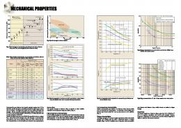
Results Figures 1, 2 and 3 present the results of the computed cost-functions. The values of the color scale are displayed in decibels in order to avoid that small amplitudes variations are hidden by very large values of the cost function. Nine observables have been evaluated, they can be ranked into 3 different categories : the phase observables (figures 1) , the V/H observables (figures 2) and the V/T observables (figures 3). The costs functions phase observables for multicomponent data, for the vertical component only or for the horizontal component show a similar behavior : the isovalues of the cost functions show a decreasing sensitivity of the depth of the interface, with respect to the depth parameter. One immediate consequence: when using a local minimization algorithm if the starting model considers an interface too deep, then the inversion will probably fail to recover the correct depth of interface. Another problematic point is the occurrence of local minima in the region of the cost function with the lowest values (-30dB to -35dB) so that a local minimization algorithm may be blocked without converging to the global minima. If we compare the results, using the polarization attribute of the V/H ratio, it can be shown that all the different versions (with complex value, amplitudes and phase) of the V/H ratio based cost functions show a global minimum centered in the right model space position. Another remarkable point is the higher dynamic range of the cost function, in all the cases for polarization observables is at least of 60 dB. However, when dealing with deep area (deeper than 10m) the cost functions show also a relative insensitivity to the depth of the layer. The cost functions based on the V/T ratio present a similar behavior as those based on the V/H ratio. Misfit computed with the phase, all components
Misfit computed with the phase, vertical component only
0
0
Misfit computed with the phase, horizontal component only
0
-10
-5
-5
-20 -10
-15
10
-40
10
-20
-25
15
-10
5 -30
Depth of the top layer (m)
5
Depth of the top layer (m)
Depth of the top layer (m)
5
-15
10
-50 -60
15
-30
-20
15
-25
-70 -30
20 350 400 450 500 550 600 650 Shear wave velocity of the top layer (m/s)
20 350 400 450 500 550 600 650 Shear wave velocity of the top layer (m/s)
-35
(a) Phase using all the component
-80
20 350 400 450 500 550 600 650 Shear wave velocity of the top layer (m/s)
(b) Phase using only the vertical component (c) Phase using only the horizontal component
Figure 1 Cost functions computed with the phase (values in dB) Misfit based on the VH ratio
Misfit based on the amplitude of VH ratio
0
Misfit based on the phase of the HV ratio
0
0 -10
-10
-20
-20
10
-40
-50
15
-20
5 -30
-40
10
-50
15
-60
Depth of the top layer (m)
-30
5
Depth of the top layer (m)
Depth of the top layer (m)
5
-10
-30
10 -40
15
-50
-60 -70 20 350 400 450 500 550 600 650 Shear wave velocity of the top layer (m/s)
-70
(a) V/H ratio
20 350 400 450 500 550 600 650 Shear wave velocity of the top layer (m/s)
(b) V/H ratio amplitude
-60 20 350 400 450 500 550 600 650 Shear wave velocity of the top layer (m/s)
(c) V/H ratio phase
Figure 2 Cost functions computed with the VH ratio (values in dB)
Conclusions and perspectives In this study, several observables have been investigated for FWI in near surface context for a simple case. We showed that cost functions based on the phase observables present two main issues : the occurrence of local minima and regions of indetermination when the depth of the interface increases. In 75th EAGE Conference & Exhibition incorporating SPE EUROPEC 2013 London, UK, 10-13 June 2013
Misfit based on the VT ratio
Misfit based on the amplitude of the VT ratio
0
0
Misfit based on the phase of the VT ratio
0
-10
-10
-10
-20
-20
-40
10
-50
15
-60
-20
5 -30 -40
10
Depth of the top layer (m)
-30
Depth of the top layer (m)
5
Depth of the top layer (m)
5
-30
10
-50 -60
15
-40
-50
15
-70 -60
-70 20 350 400 450 500 550 600 650 Shear wave velocity of the top layer (m/s)
(a) V/T ratio
20 350 400 450 500 550 600 650 Shear wave velocity of the top layer (m/s)
(b) V/T ratio amplitude
-80
20 350 400 450 500 550 600 650 Shear wave velocity of the top layer (m/s)
(c) V/T ratio phase
Figure 3 Cost functions computed with the VT ratio (values in dB) this case, we have shown that the cost functions based on the V/H ratio or on the V/T ratio can provide additional constraints to reach the true model due to well convex shape of the cost functions associated to these observables. Some other considerations are currently under investigation. First the robustness of cost-functions to measurement noise. Furthermore it will be interesting to study the behavior of these cost functions when attenuation parameters are not properly known, or in case of source amplitude errors (2D/3D) and or strong source distortions. Other tests are also currently conducted in order to evaluate the effectiveness of this approach with strong velocity contrasts. The implementation of these observable in the gradient of the FWI method is relatively straightforward but perhaps one difficult point will be the design and setup-up of a cost function combining phase and polarization observables.
Acknowledgements The first author (R. Valensi) highly appreciated discussions with J. Virieux and F. Treyssede and he is thankful to I. Masoni for her assistance in accessing CIMENT resources. Authors thank M. Dietrich for providing his numerical modeling code (Dietrich, 1988). This work was produced using the CIMENT high-performance computing facilities (Université Joseph Fourier, Grenoble).
References Arai, H. and Tokimatsu, K. [2005] S-wave velocity profiling by joint inversion of microtremor dispersion curve and horizontal-to-vertical (h/v) spectrum. Bulletin of the Seismological Society of America, 95(5), 1766–1778, doi:10.1785/0120040243. Barnes, C. and Charara, M. [2010] Constrained full-waveform inversion of multi-component seismic data. 72nd EAGE Conference and Exhibition, Barcelona. Bodet, L. et al. [2005] Surface-wave inversion limitations from laser-doppler physical modeling. Journal of Environmental & Engineering Geophysics, 10, 151–161. Boore, D.M. and Nafi Toksoz, M. [1969] Rayleigh wave particle motion and crustal structure. Bulletin of the Seismological Society of America, 59(1), 331–346. Bretaudeau, F., Brossier, R., Leparoux, D., Abraham, O. and Virieux, J. [2013] 2d elastic full waveform imaging of the near surface : Application to a physical scale model. Near Surface Geophysics. Dietrich, M. [1988] Modeling of marine seismic profiles in the t-x and tau-p domains. GEOPHYSICS, 53(4), 453–465. Ellefsen, K.J. [2009] A comparison of phase inversion and traveltime tomography for processing near-surface refraction traveltimes. GEOPHYSICS, 74, WCB11–WCB24. Leki´c, V. and Romanowicz, B. [2011] Inferring upper-mantle structure by full waveform tomography with the spectral element method. Geophysical Journal International, 185(2), 799–831. Muyzert, E. [2009] Surface wave spectral ratio inversion for shear velocity. 71nd EAGE Conference and Exhibition, Amsterdam. Sears, T., Barton, P. and Singh, S. [2010] Elastic full waveform inversion of multicomponent ocean-bottom cable seismic data: Application to alba field, u. k. north sea. GEOPHYSICS, 75(6), R109–R119. Tanimoto, T. and Rivera, L. [2008] The zh ratio method for long-period seismic data: sensitivity kernels and observational techniques. Geophysical Journal International, 172(1), 187–198. Virieux, J. and Operto, S. [2009] An overview of full-waveform inversion in exploration geophysics. GEOPHYSICS, 74(6), WCC127–WCC152.
75th EAGE Conference & Exhibition incorporating SPE EUROPEC 2013 London, UK, 10-13 June 2013