non-parametric bootstrap confidence interval for median. ExamplEs. To illustrate the examples of sample mean and sample median statistics as mentioned.
Statistics
Introduction to Bootstrap Stephanie Fook Chong1,2, MSc, CStat, Robin Choo3, BSc Department of Clinical Research, Singapore General Hospital, Singapore Centre for Quantitative Medicine, Office of Clinical Sciences, Duke-NUS Graduate Medical School, Singapore 3 Singapore Institute for Clinical Sciences, A*STAR, Singapore 1 2
A fundamental issue in statistics is about assessing the variability of an estimate known as the standard error (SE) of the statistics of interest. Drawing different samples from the same population will yield different estimates; this hypothetical set of estimates represents the sampling distribution of the statistics. However, in real life, it is not possible to repeat the study many times. Before the widespread availability of fast computers, sampling distribution of a statistics was derived mathematically. The mathematical derivations usually require assumptions about the distribution of the data and apply only to certain statistics such as mean. One way of repeatedly drawing samples many times from a dataset is via the aid of fast computers which are easily available nowadays. This process of drawing large number of samples from the dataset and subsequently making numerical calculations to infer the sampling distribution of an estimate is known as resampling. Various resampling techniques exist. The bootstrap, jackknife, cross-validation and monte-carlo simulation are examples of such techniques. All these techniques have the advantage of not necessitating any assumption about the distribution of the data nor requiring specialised training in statistics. On the other hand, there are also critics who question the accuracy of the estimate obtained by the resampling techniques because the same numbers in the sample are used again and again . The argument is that the technique is limited by the size of the sample dataset and its representativeness of the population. In this article, we will focus on a
236
short introduction to the bootstrap. It is hoped that both junior biostatisticians and clinicians who wish to obtain a better appreciation of the mechanics behind bootstrapping will find this article useful. Bootstrapping is a computer-based technique that can be used to infer the sampling distribution of almost any statistics via repeated samples drawn from the sample itself, as opposed to the hypothetical resampling from the population. The phrase “to pull oneself by one’s bootstrap” is widely thought to be based on the famous story Adventures of Baron Munchausen by Rudolph Erich Raspe. According to the stories, the Baron had fallen into a swamp and saved himself by pulling himself up by his own bootstraps. When no simple formula for the computation of SE exists, bootstrapping is particularly useful. In this article we aim to provide a brief illustration of the mechanism of bootstrapping for the computation of SE of mean, SE of median and non-parametric bootstrap confidence interval for median. Examples To illustrate the examples of sample mean and sample median statistics as mentioned earlier, a random sample of the weight of 25 adults in kilogrammes (kg) will be drawn from a dataset of 1,000 population-based individuals recruited under the Singapore Thyroid and Heart Study (THS)1. For our illustration, we treat the later dataset as the population and Table 1 (overleaf ) is the random sample that was selected.
Proceedings of Singapore Healthcare Volume 20 Number 3 2011
Introduction to Bootstrap Table 1. Random sample of 25 weights (kg) from 1000 subjects of Singapore Thyroid and Heart Study (ordered from lowest to highest). 38.5
40.5
40.8
44.9
45.0
45.0
47.0
48.0
48.1
48.8
55.2
58.5
58.5
62.5
63.4
49.2
49.5
50.9
53.1
54.9
66.2
69.7
70.1
70.5
77.9
Standard error of sample mean For the data in Table 1, the sample mean is given by 1
=
•Υ
n
n
Σ Υ = 54.27. i
i=1
And, from statistical theory we know that the sampling distribution of•Υ, also known as sampling error of mean is SE =
SD = 2.14 √ •n
where SD =
n
1
√
n–1
Σ (Υ –•Υ) i
2
= 10.69
i=1
and the sample size, n = 25. The above formula for SE arises from the Central Limit Theorem that says that•Υ is approximately normally distributed. We’ll now proceed to show how non-parametric bootstrap can be used as an alternative method to compute the sampling distribution of the mean. The data from Table 1 is treated as if it was a population and a random sample of size n = 25 with replacement of values allowed, is drawn from it. This step is known as a bootstrap resample. A second, third, fourth and more resamples can be drawn from Table 1. Table 2 (overleaf ) represents 1,000 bootstrap resamples from data in Table 1. The statistics of interest, the sample mean is calculated and displayed for each bootstrap resample in Table 2. The bootstrap method of computing SE of mean is given by SEBS
=
√
1
1000 – 1
1000
( –•Υ ) = 2.09, Σ •Υ 2
i=1
where•Υi is the mean of bootstrap sample i and•Υ is the grand mean of all the bootstrap means.
As can be seen, the bootstrap standard error of 2.09 is very close to the standard error of 2.14 obtained earlier, using theoretical formula. This is especially so with large number of resamples, as in our case whereby we did the 1,000 resampling. For estimating a standard error, it is sufficient to use from 50 to 200 replicates as can be seen in Table 3 (overleaf ). The same bootstrap technique as described above is used to generate 1,000 resamples with replacement from the population. This process is done in order to obtain the true sampling distribution of the mean and is displayed in the left panel of Fig. 1 (overleaf ). The right panel of Fig. 1 shows the distribution of the 1,000 bootstrap means of Table 2 and is a bootstrap estimate of the true distribution in the left panel. The 2 panels are very similar but with differences resulting from the step that uses the sample as if it was the population for drawing random samples that are used to generate the right panel of Fig. 1. This step is referred to as the bootstrap step. Standard error of sample median Unlike the sample mean, there is no simple expression for the standard error of the sample median. Bootstrapping provides the simplest way to compute the sampling distribution of the sample median. Just as for the sample mean, the sample median is calculated and displayed for each bootstrap resample in Table 2. The median for our sample in Table 1 is 50.9. Just like for the sample mean, bootstrap technique is used to generate 1,000 resamples with replacement from the population in order to obtain the true sampling distribution of the median in the left panel of Fig. 2 (following page). Following the same analogy as for Fig. 1, the right panel of Fig. 2 shows the distribution of the 1,000 bootstrap medians of Table 2 and is a bootstrap
Proceedings of Singapore Healthcare Volume 20 Number 3 2011
237
Statistics Table 2. Bootstrap resamples B1 to B1000 drawn from Table 1. 1
Sample
B1
B2
B3
B4
B5
…
B1000
38.5
40.5
63.4
70.1
62.5
47.0
…
69.7
2
40.5
70.5
70.5
49.5
45.0
70.5
…
50.9
3
40.8
63.4
50.9
48.0
48.0
70.1
…
58.5
4
44.9
38.5
70.1
63.4
40.5
45.0
…
38.5
5
45.0
6
45.0
…
48.1
66.2
38.5
66.2
58.5
…
48.1
48.1
48.1
38.5
58.5
47.0
…
49.2
…
…
…
…
…
…
…
…
…
22
69.7
58.5
77.9
77.9
55.2
70.1
…
69.7
23
70.1
58.5
55.2
38.5
53.1
40.5
…
40.5
24
70.5
45.0
47.0
54.9
49.2
49.5
…
40.5
25
77.9
44.9
50.9
63.4
48.8
45.0
…
55.2
Mean
54.3
53.1
54.4
55.8
54.2
54.5
…
51.9
Median
50.9
49.5
49.5
54.9
49.5
49.5
…
50.9
Table 3. Standard error of sample mean and sample median and, corresponding bootstrap standard errors for replicates ranging from 50 to 1,000,000. Bootstrap replicate numbers Sample
50
100
200
500
1,000
10,000
100,000
1,000,000
SEmean
2.14
2.01
2.06
2.08
2.12
2.09
2.10
2.09
2.09
SEmedian
?
3.06
3.10
2.97
3.14
3.17
3.17
3.16
3.16
Fig. 1. (Left) Histogram of 1,000 sample means from repeated sampling of the population of 1,000 subjects. (Right) Histogram of 1000 bootstrap sample means from randomly sampling with replacement from Table 1 data.
238
Proceedings of Singapore Healthcare Volume 20 Number 3 2011
Introduction to Bootstrap
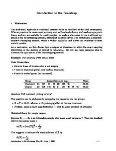
Fig. 2. (Left) Histogram of 1,000 sample medians from repeated sampling of 1000 subjects. (Right) Histogram of 1,000 bootstrap sample medians from randomly sampling with replacement from Table 1 data.
estimate of the true distribution in Fig. 2’s left panel. It can be noted that the maximum frequency count (as read from the y-axis) in the 2 panels of Fig. 2 differ substantially. The dissimilarity between the 2 panels of Fig. 2 stems from the bootstrap step that treats the sample as a pseudo-population and the nature of the median which takes on discrete values as opposed to continuous values, overall resulting in the sampling distribution in the right panel of Fig. 2 being very discrete. However, we can say that the 2 panels of Fig. 2 are similar in shape, albeit not as similar as the 2 panels of Fig. 1. Visual comparison of Fig. 1 and 2 reflect the fact that the sampling distribution of the sample median is more difficult to estimate than that of the sample mean. The bootstrap standard error of the median which is in fact the standard deviation of the bootstrap medians is SEBS
=
√
1 1000 – 1
1000
Σ (Μˆ –•Μ)ˆ
2
= 3.17,
i=1
where Μ ˆ is the median of bootstrap sample i and •Μ ˆ is the grand mean of all the bootstrap medians.
Nonparametric bootstrap confidence interval In most circumstances, confidence interval (CI) for an estimate is calculated from the observed quantity of interest (e.g. mean), the standard normal z-score and the SE of the estimate. However, there is no simple formula for SE of median. This problem can be circumvented by using the bootstrapping technique. Generation of confidence interval is an important statistical technique amenable to bootstrap. In this section we will show how to construct one of the simplest bootstrap approaches to confidence interval, the bootstrap percentile interval. The 1,000 median estimates from the 1,000 resamples in Table 2 is sorted in ascending order and thus denoted by M(1), M(2), ... , M(1,000). A 95% bootstrap percentile interval is then given by (M(25), M(975)) = (48.1, 58.5). Conclusion Bootstrap is a computationally intensive technique, especially useful for estimating the precision of an estimate when there is no simple formula associated with the sampling error of the sample statistics. The method can be applied to any estimator, whether simple or complicated. As long
Proceedings of Singapore Healthcare Volume 20 Number 3 2011
239
Statistics
as a computer program for resampling is available, a 95% confidence interval is easily obtained from a 95% bootstrap percentile interval.
understanding of the topic of bootstrap can refer to the book by Efron et al2.
Usage of bootstrapping techniques is de rigueur in areas such as genetic association studies and clinical prognostic model validation. This article only provides a glimpse of the many applications of the bootstrap technique. Biostatistics practitioners and clinician scientists wishing to have a wider
1. Hughes K, Yeo PP, Lun KC, Thai AC, Sothy SP, Wang KW, et al. Cardiovascular diseases in Chinese, Malays, and Indians in Singapore. II. Differences in risk factor levels. J Epidemiol Community Health. 1990;44(1):29–35. 2. Efron B, Tibshirani RJ. An introduction to the bootstrap. 1st ed. New York: Chapman & Hall; 1993. 456 p.
References
240
Proceedings of Singapore Healthcare Volume 20 Number 3 2011