Introduction to error correcting codes in quantum computers - SciELO

˜ ENSENANZA

REVISTA MEXICANA DE F´ISICA E52 (2) 218–243

DICIEMBRE 2006

Introduction to error correcting codes in quantum computers P.J. Salas-Peralta Departamento de Tecnolog´ıas Especiales Aplicadas a la Telecomunicaci´on, Universidad Polit´ecnica de Madrid, Ciudad Universitaria s/n, 28040 Madrid, e-mail: [email protected] Recibido el 25 de octubre de 2005; aceptado el 7 de marzo de 2006 The goal of this paper is to review the theoretical basis for achieving a faithful quantum information transmission and processing in the presence of noise. Initially, encoding and decoding, implementing gates and quantum error correction will be considered error-free. Finally, we shall relax this non-realistic assumption, introducing the quantum fault-tolerant concept. The existence of an error threshold permits us to conclude that there is no physical law preventing a quantum computer from being built. An error model based on the depolarising channel will be able to provide a simple estimate of the storage or memory computation error threshold: ηth < 5.2 10−5 . The encoding is made by means of the [[7,1,3]] Calderbank-Shor-Steane quantum code, and Shor’s fault-tolerant method is used to measure the stabiliser’s generators. Keywords: Quantum error correcting codes; decoherence; quantum computation. El objetivo de este art´ıculo es la revisi´on de los fundamentos te´oricos que permiten una correcta transmisi´on y procesado de la informaci´on cu´antica en presencia de ruido. Inicialmente, los procesos de codificaci´on, decodificaci´on, aplicaci´on de puertas y correcci´on de errores se considerar´an sin error. Finalmente relajaremos esta consideraci´on no realista, lo que conducir´a al concepto de tolerancia a fallos. La existencia de un umbral de error permite concluir que no hay ninguna ley f´ısica que impida construir un ordenador cu´antico. Mediante un modelo de error basado en un canal despolarizante, se har´a una estimaci´on simple para el umbral de los errores de memoria: ηth < 5.2 10−5 . La codificaci´on se realiza mediante un c´odigo cu´antico [[7,1,3]] de Calderbank-Shor-Steane, y se usa el m´etodo de Shor tolerante a fallos para medir los generadores del estabilizador. Descriptores: C´odigos correctores de errores cu´anticos; decoherencia; computaci´on cu´antica. PACS: 0367-a; 0367Lx

1. Introduction Quantum Mechanics (QM) has traditionally been used to study microscopic systems, achieving unquestionable successes in such varied fields as atomic structure, elementary particles, solids, liquids, molecules, nuclei, radiation, etc. It is currently expanding into a field traditionally dominated by a classic description: Computation and Information Theory. Although the devices making up a classic computer work according quantum laws, they do not make use of the quantum representation of the information, but they still use the classic version: bits. The recognition that the information is closely related to its physical representation, and the non-local character of the QM, is opening up an unsuspected perspective from a classic point of view for data processing [1]. In this context, the concept of the quantum computer appears to be a device that takes advantage of the quantum evolution to obtain new forms of information processing. Its minimum unit of information is the quantum bit or qubit, that consists of a state (coherent superposition of two others representing the classic possibilities |0i and |1i) of the type |qi = a|0i + b|1i, where a and b are complex numbers. Like classic computers, quantum computers experience the presence of noise that induces errors in them. Unlike classic computers,quantum ones must handle coherent superposition and entangled states, allowing interference phenomena analogous to those produced when light crosses a system of

two slits of a size compareble to its wavelength. Unfortunately, the superposition of states is extremely sensitive to noise and they are easily destroyed due to an uncontrollable interaction with the environment. This process is known as decoherence [2]. It would be possible to think about eliminating it by improving the isolation of the device. Nevertheless, the extraction of the information at the end of any computation process always implies some type of measurement; this is why simple isolation is not a solution. In addition, it is impossible to completely eliminate all the interactions that come from the environment. Until 1995, it was believed that the unavoidable decoherence would prevent the quantum information processing from showing its advantages with respect to the classic case. Luckily, things were going to change [3]. The objective of the present paper will be to show how noise is not an unsolvable problem in building a quantum computer. After a brief introduction to classic error correction, the characteristics of quantum errors are introduced, and the noise effect will be exemplified by means of the Grover algorithm including five qubits. Several strategies introduced to control the decoherence will be reviewed, focusing the explanation on the quantum error correcting codes. A simple numerical method, encoding a qubit by means of the [[7,1,3]] fault-tolerant quantum code, permit us to infer the existence of an error threshold below which a sufficiently long quantum computation would be possible. Finally, concatenated codes will promise to improve error correction capabilities.

INTRODUCTION TO ERROR CORRECTING CODES IN QUANTUM COMPUTERS

2.

Classic errors and their correction

In order to understand the main ideas in quantum error correction, we start with some classic background. Classic information is represented by means of an alphabet of p symbols. The binary alphabet (p = 2) is made up of two symbols {0, 1}, and the information contained in each symbol is called a binary digit or a bit. The information processing involves representing it as bit strings, sending them through a channel or carrying out a computation and, finally, arriving at a result. Unfortunately, noise can always corrupt the information. A possible strategy for preserving the classic information against the noise effect is by means of an encoding method. The information contained in a single bit is spread out along a bit string of length n, called the classic register or codeword. From a mathematical point of view, the set of all words of length n (V2n ), with modulo 2 arithmetic, could have a structure. Of particular importance are the sets of codewords C ⊆ V2n , which have a vector space structure, called linear codes. This structure makes the correction process easier. It is also possible to define a product operation which, together with addition, defines a finite field also called a Galois field. The binary alphabet {0, 1} is an example, and will be referred to as the GF(??) field or as vector space V2 . The Hamming distance d(u,v) between two codewords u, v ∈ C ⊆ V2n is the number of coordinates where the vectors u and v differ: d(u, v)= |{i : 1 ≤ i ≤ n, ui 6= vi }| .

(1)

The bars signify the number of elements of this set. The distance d satisfies the axioms for a metric on V2n . The minimum distance of a code is the smallest distance between two different codewords. The number of non-zero components of a binary string of V2n is called the weight (or Hamming weight, WH ), and the distance between u and v is d(u,v)=WH (u-v). The code capability to correct errors is represented by the code distance. Suppose the emitter sends the codeword u ∈ C through a classic channel affected by some error probability, and the receiver detects a slightly different codeword u’ = u+e 6= u, affected by the error e ∈ V2n . By means of the minimum distance decoder, the word u’ = u+e will be decoded as the closest codeword, according to the Hamming distance. Having a code C with distance d ≥ 2t + 1 (or d > 2t), the receiver will recognize the correct codeword u from u’ if and only if it fulfils d(u,u’) = WH (e) ≤ t, because in this case d(u,u’) < d(v,u’), ∀v ∈ C. As a result, code C with distance d will correct any word u’ = u+e, satisfying WH (e) ≤ t, and it will be a t-errorcorrecting code. Thus, good error correction means large minimum distance. On the other hand, fast transmission rate means many codewords, with a small distance between them. This tension is the basis of coding theory. To visualise the code distance and correcting capabilities, each codeword uj ∈ C is represented as the “centre” of a “sphere” with radius t = b(d − 1)/2c. The sphere

219

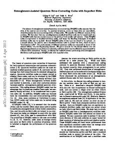
contains all binary sequences v = uj + e ∈ V2n such as d(uj ,v) ≤ t. Since code C is t-error-correcting, the spheres are disjoint. The vectors inside the t-sphere come from uj affected by an error e of weight WH (e) ≤ t. Fig. 1 shows the case d= 5 (t = 2). Any erroneous codeword u’ = u1 + e1 with WH (e1 ) = 2 is successfully corrected with a d = 5 code, but not if u’ = u1 +e2 with WH (e2 ) = 3. In this case, u’ would be wrongly corrected as u2 . If C is a vector subspace of V2n , d is the smallest weight of a non-zero codeword. Thus, a binary classic code of dimension k (including 2k codewords) of length n and minimum distance d is noted as C=[n, k, d] ⊆ V2n . A linear code [n,k,d] (i.e. a linear subspace) can be specified in either of two ways: 1) The k basis vectors of C are arranged in the k×n generator matrix G. Thus C={xG, x ∈ V2k }.

(2)

This is useful for encoding. If the messages to be transmitted are all k-tuples x over V2 , then we can encode them as the codewords xG. 2) It is possible to define a scalar (or inner) product in V2n as the standard rule of multiplying the components and making the addition modulo 2. Two vectors are orthogonal if their scalar product is zero. The code can also be determined as the subspace orthogonal to some predetermined set of vectors. Each orthogonality condition divides the space in two, and then we can specify a code having 2k vectors (and dimension k), through its orthogonality to (n-k) vectors. These vectors can be arranged as an (n-k)×n matrix, called parity-check matrix HC , and the code can be specified as C = {v ∈ V2n , HC v T = 0}.

(3)

This is useful for error correction. The set of correctable errors S must satisfy: ∀ei , ek ∈ S ⊆ V2n , ∀ u, v ∈ C, if u 6= v

F IGURE 1. Geometrical representation of a classic code with distance 5. Each codeword uj (black squares) is at the “centre” of a “sphere” with radius t = 2. An erroneous codeword (unfilled square) u’ = u1 + e1 with WH (e1 ) = 2 is successfully corrected as u1 . If WH (e2 ) = 3 the codeword u’ = u1 + e2 is wrongly corrected as u2 .

Rev. Mex. F´ıs. E 52 (2) (2006) 218–243

220

P.J. SALAS-PERALTA

then u + ei 6= v + ek . If vector u + ei is detected, the receiver can correctly infer the codeword u. This process is very easy for linear codes using the parity-check matrix. Suppose the receiver detects vector u + e, with u ∈ C and e ∈ S. Applying the parity-check matrix HC , HC (u + e)T = HC uT + HC eT = HC eT . The vector HC eT = s 6= 0, having (n-k) components, characterizes the error; it is called the error syndrome and does not depend on u. Because the total number of syndromes is 2n−k , the code can correct the same number of different errors. If we can deduce the error e from its syndrome, the correction is immediate. Even though a classic code is not necessarily a vector space, in this paper we shall be concerned only with linear codes. A simple classic code is the repetition code in which the 0 bit is encoded by copying the bit three times as a codeword (000), and the bit 1 is encoded as the string (111). The set of all codewords of length three span a vector space, and the set {(000), (111)} is a basis of a two-dimensional subspace C ⊆ V23 . This subspace C is our classic repetition code of length three. The code {(000), (111)} can be specified as the subspace orthogonal to (110) and to (101), and both vectors written as a 2×3 matrix form the parity-check matrix HC , and the code satisfies the condition ∀u ∈ C, HC uT = 0. The 1×3 generation matrix G is (111). Clearly the code has distance three, so is written as [3,1,3]. If we want to send a bit 0 through a noisy channel, using the repetition code, we send (000). Classic noise appears as bit-flip errors, and can be represented as error codewords of V23 . If the channel introduces a bit-flip error (with a probability ε) into the third bit, e = (001), it will be enough for the receiver to watch the three bits, and finding the syndrome (01), it will suppose that an error in the third copy has occurred, recovering the bit to replace the (000) (majority voting decoding). For this method to be advantageous, it is necessary for the probability of correct transmission (1-ε) of each bit to be higher than 50%, otherwise the majority voting method would provide an erroneous answer. A wrong decoding will occur if the received word has two 1’s. Given a parity-check matrix, each of its columns represents the syndrome for an error. If all the columns are different, the code can correct one bit-flip and is called Hamming code whose general parameters are [2r -1, 2r -1-r, d] with r ≥ 2. An example that will be used in the quantum construction is [7,4,3]. This code has a subcode C⊥ ⊂ C whose codewords of even weight are orthogonal (with respect to the scalar product) to those of C. In general, given a code C=[n,k,d], its orthogonal or dual code is C⊥ =[n, n-k, d⊥ ]; and if C ⊂ C⊥ , it is said that C is weakly self-dual, and if C=C⊥ , C is self-dual. The property of weak self-duality will be used in the quantum error correcting code construction. Besides the Hamming codes, Reed-Muller codes are an interesting family of weakly self-dual and self-dual codes. Their

parameters are: · µ ¶ µ ¶ m m RM (r, m) = n = 2m , k = + 0 1 µ ¶ ¸ m +··· + , 2m−r , (4) r with 0 ≤ r ≤ m. Other classic codes can be created be means of different scalar products and higher alphabet dimensions. There are several bounds related to classic codes. One of them is the Hamming bound reflecting that a code C = [n,k,d] with block length n can correct errors of weight t if there is enough room in the total vector space (of dimension n) to accommodate the errors: Number of different errors ¶ t µ X n = ≤ 2n−k i i=1

= total number of different syndromes

(5)

Let the codewords be {ui , i=1,. . . ,2k }. For each codeword we can draw a “sphere” with “centre” at uj and “radius” t. The sphere contains all binary sequences v such as d(uj ,v) ≤ t. Since the code C is t-error-correcting, the spheres are disjoint. The summation in Eq. (??) is the number of v = uj + e vectors inside the t-sphere coming from uj , affected by an error e of weight WH (e) ≤ t. In order to differentiate errors, this value must be smaller than the number of different syndromes. A code is perfect if it attains the equality in (??), and the union of all the spheres is V2n .

3.

Origin of quantum errors

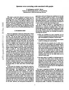
All of the systems are subject to noise of diverse origins (interaction with the environment, incorrect application of gates, etc.), giving rise to errors. In order to carry out a quantum computation, it is necessary to eliminate or control these errors. Focusing on the quantum computation, and from the point of view of their origin, these errors can be internal and external (Fig. 2). The internal ones appear even if there is no interaction with the environment and originate in the faulty operation of some parts of the hardware. Several types of them include:

F IGURE 2. Framework of the different error sources in a quantum computer.

Rev. Mex. F´ıs. E 52 (2) (2006) 218–243

221

INTRODUCTION TO ERROR CORRECTING CODES IN QUANTUM COMPUTERS

4.

1) Errors in the preparation of the initial states Classically the errors appearing in the preparation of the initial state propagate exponentially with respect to the number of steps; nevertheless, from a quantum point of view, they are constant. Let us suppose that we prepare an initial state |ψi i evolving by means of a ˆ (or an evoprocess characterised by a Hamiltonian H ˆ −iHt ˆ lution operator U = e , h/2π=1) until reaching the final state |ψf i. In the case of a perfect preparation, ˆ ˆ (t) |ψi i = e−iHt |ψi i → |ψf i = U |ψi i

(6)

If the initial state corresponds to a set of single qubits, all of them in the state |0i except the k qubit having an error ε, ³p ´ |ψi i= |0i ⊗ |0i ⊗...⊗ 1−ε2 |0k i +ε |1k i ⊗...⊗ |0i p = 1 − ε2 |ψi i + ε |wastei (7) and its time evolution will be: p ˆ |ψi i + εU ˆ |wastei |ψf i = 1 − ε2 U p = 1 − ε2 |ψf i + ε |dirty wastei ,

Problems in the correction of quantum errors

At the time of designing methods to control quantum errors, the following question arises; can we apply classic strategies to the quantum systems? For example, could classic error correcting codes be used? The answer to this question has been negative because of the following problems: 1. Continuous errors Classically, the only permissible errors are those of bit-flip (transformation of a bit 0 to 1 or the reverse) and are discrete, but for the quantum case the situation is more complicated. The errors can affect the modules of the coefficients a and b in the qubit superposition (amplitude decoherence), as well as its relative phases (phase decoherence), both being continuous ones. For instance, if the physical representation of qubits implies that |0i is the fundamental state of an atom, whereas |1i corresponds to an excited state, a spontaneous decaying process produces an amplitude decoherence. Its time evolution will be

(8) 2

which implies that the initial error (given by |ε| in |ψi i) does not increase in the evolution. This behaviour arises from the linearity of the QM. In some cases, the quantum algorithms are even sensitive to these errors in the amplitude, and their accumulation becomes dangerous. It is necessary to pay special attention when the initial errors affect, not the amplitude, but the relative phases [?], whose effect depends on the quantum algorithm considered. 2) Hardware errors Their origin is in the noisy gate application, especially when they are analogical (working with continuous parameters) and can be described as unitary errors due to an error term ηˆ in the noiseless Hamiltonian ˆ 0 :H ˆ η =ˆ ˆ 0 . The noiseless evolution is H η +H ˆ0t −iH e |ψi i=|ψf i. If the error operator ηˆ is small ˆ 0 , ηˆ] ∼ enough, [H = 0 and the ηˆ effect on |ψi i is ˆ 0 )t −i(ˆ η +H e |ψi i = e−iˆηt |ψf i. The exponential can be expanded and only retain the linear term, and |ψi i evolves to (1 − iˆ η t) |ψf i. So the error probability becones quadratic in time. 3 Read-out errors of the results at the end of the process Related to the amplification of the results from the quantum domain to the classic macroworld. In addition to the internal errors, external ones may appear because the system is not completely isolated from its environment, leading to a decoherence, and giving rise to a non-unitary evolution of the states in the quantum computer. This loss of coherence is the most serious problem which future quantum computers face.

©

1

|q(t)i = q

2

2

ª a |0i +be−γt |1i . (9)

|a| + |b| e−2γt In the case where it only affects its relative phase, the qubit is transformed into (a|0i+beiφ |1i). If φ=π, we have a discrete phase-flip error, analogous to the classic bit-flip. The phase-flip is only a quantum error. 2. Impossibility of introducing redundant information copying it One of the ideas on which the correct transmission of classic information is based, is the possibility of copying it (introducing redundancy), which allows information recovery in the presence of noise as indicated in Sec. 2. Unfortunately, quantum mechanically it is not possible to copy unknown qubits perfectly, due to the impossibility of cloning unknown qubits [5]. In order to copy a qubit, we need to know about it. Given a qubit |qi=a|0i+b|1i (with unknown coefficients a and b), we would have to measure it to obtain the a and b values, but in doing so we would produce its collapse, destroying it irreversibly. 3. Measurement problem In order to correct the errors, we must measure the state of the system (for example some qubits) to find out what type of error has occurred. When doing so, the state collapses with the consequent irreversible loss of information. In the following sections we shall review the way in which all these problems were solved.

Rev. Mex. F´ıs. E 52 (2) (2006) 218–243

222

P.J. SALAS-PERALTA

5. Discretization of quantum errors In 1995, the way was discovered to transform typically continuous quantum errors, in discrete solving the first aforementioned problem. The strategy consists of embedding the {environment + qubit} continuous evolution only in the first, making a discrete description of the qubit state evolution. Formally the interaction process of a qubit with its environment can be described by means of the following evolution [?]:

ˆ (t) U

µ Iˆ ≡ µ Yˆ ≡

1 0

¶

0 1

µ ˆ≡ X

,

0 −1 1 0

¶ =−iσY ,

¶ 1 = σX 0 µ ¶ 1 0 ˆ Z≡ =σZ (12) 0 −1

0 1

sometimes called the canonical set of errors, whereas the states of the environment are:

ˆ (t) U

|0i |ei −→ c00 |e0 i |0i + c01 |e1 i |1i |1i |ei −→ c10 |e0 i |0i + c11 |e1 i |1i

ˆ X, ˆ Yˆ , Zˆ are States |ei i describe the environment, and I, the operators whose representation in terms of the Pauli matrices {I, σX, σY , σZ } is:

(10)

{|0i, |1i} being the qubit states and |ei the initial state of the environment. The total initial state is the tensor product of the qubit and the environment states, and evolve (unitarily) by means of the coefficients cij that depend on the noise. This is the most general form of the noise effect, assuming that qubits do not leave the two-dimensional {|0i, |1i} subspace of the total Hilbert space H2 . The qubit evolution whose initial (t = 0) state is |q(0)i = a|0i + b|1i can be expressed as: ˆ (t) U

|q(0)i |ei = (a |0i + b |1i) |ei −→ |ψ(t)i n o ˆ |eX i X+ ˆ |eY i Yˆ + |eZ i Zˆ |q(0)i . (11) = |eI i I+

1 (c00 |e0 i + c11 |e1 i) 2 1 |eX i = (c10 |e0 i + c01 |e1 i) 2 1 |eY i = (c01 |e1 i − c10 |e0 i) 2 1 |eZ i = (c00 |e0 i − c11 |e1 i) 2 |eI i =

The state |ψ(t)i reflects a correlation between the states of the environment and those of the qubit, describing a mixed state that has lost some coherence. If we could make a measurement on the joint state vector |ψ(t)i of the {environment + qubit} conserving the qubit coherence, we would collapse the state into one of the following terms:

 |eI i Iˆ |q(0)i = |eI i { a |0i + b |1i} → State without error    ˆ |q(0)i = |eX i { a |1i + b |0i} → Bit - flip error |eX i X M easure |ψ(t)i −→  |e i Zˆ |q(0)i = |eZ i { a |0i − b |1i} → Phase - flip error   Z |eY i Yˆ |q(0)i = |eY i { a |1i − b |0i} → Phase and bit - flip error with a collapse probability given by ¯ ¯ ¯2 ³ ´ ¯ ¯ 2 ˆ ˆ ¯ |εi | = ¯hq(0), ei | Aˆ+ i ⊗ I U (t)¯ q(0), ei¯ ˆ X, ˆ Yˆ , Z}. ˆ Note that |εi |2 imply the overlap and Aˆi ∈ {I, between the environment states (generally neither orthogonal nor normalised), and their value can depend on time by ˆ (t). Process (??) has a fundamental importance means of U for several reasons: The complete qubit evolution can be expressed by means of four basic operators, providing a discrete translation of the noise effect. It could be said that the qubit evolution is repreˆ phase-flip (Z) ˆ and both sented via three errors: bit-flip (X), ˆ jointly (Y ). This fact shows that the matrices are a basis for the 2×2 matrices. For the same reason, the errors coming from unitary evolutions can be interpreted in this form, being able to work without the environment states explicitly. In fact, for the error identification to be complete, the environment states must be orthogonal. The noise is independent of the qubit state considered, which allows its initial coherence to be maintained after the measurement step.

(13)

(14)

This state is the front door to the error correction process. If we have some way of recognising which state we have obtained by measuring |ψ(t)i, the error correction is immediate, by simply applying the inverse transformation of the detected error, since they are unitary.

6. Independent Error model The classic error model (or channel) par excellence considers the errors in different bits as independent. Even if this model does not exactly fit reality, it can provide some valuable consequences. In QM it is possible to introduce an analogous noisy channel, called a depolarising error model, in which the environment states {|ei i, i=I,X,Y,Z} are orthogonal and its scalar product is |hei |ej i|2 =δij ε/3(i, j 6= I), where ε/3 is the probability (constant) of one of the three possible errors taking place, whereas the probability of no error is |heI |eI i|2 = (1 − ε). The qubit evolution can be represented ˆD : by means of the operator U

Rev. Mex. F´ıs. E 52 (2) (2006) 218–243

INTRODUCTION TO ERROR CORRECTING CODES IN QUANTUM COMPUTERS

ˆD (|q(0)i ⊗ |ei) U r h ½ i¾ p ε ˆ ˆ ˆ ˆ = |eX i X + |eY i Y + |eZ i Z (1 − ε) |eI i I + 3 × |q(0)i .

(15)

The error model is not completely unrealistic if one assumes that single qubits are located at well-separated spatial positions, as in an ion-trap realization of a quantum computer. As much as we are interested in handling and transmitting quantum information just as if we consider the possibility of some type of encoding, we will handle sets of n qubits called quantum registers |q1 q2 . . . qn i. To see how the decoherence affects the registers, we can make some hypotheses about the error model to simplify the problem and constitute an approach to reality [7]: 1. Locally independent errors If the environments to which the qubits are connected (at the same time step) are different and not correlated, the errors in different qubits will be independent.

223

2. Sequentially independent errors The errors in same qubit during different time steps are not correlated. 3. We assume a small qubit-environment interaction 4. Error-scalability independence The qubit error probability is independent of the number of qubits used in the computation. Under these hypotheses, errors that affect an increasing number of qubits are less probable, and the error operators for an n-qubit register are the tensor product of those onequbit operators: Aˆ{i1 ,i2 ,...,in } = Aˆ1i1 ⊗ Aˆ2i2 ⊗ . . . ⊗ Aˆnin ,

(16)

where the superscript refers to the qubit, and the subscript varies from 1 to 4: Aˆm im (for the m qubit) ∈ {I(im =1), σX (im =2), -iσY (im =3), σZ (im =4)}. In the depolarising error model, the evolution of an n-qubit quantum register is:

r ³ ´ ε (1 − ε)n/2 Iˆ1 ⊗ · · · ⊗ Iˆn |e0 i + (1 − ε)(n−1)/2 3

½ ˆD (|q1 q2 · · · qn i |ei) = |Ψ(t)i = U

o ³ ε ´n/2 X n ¯ ® Aˆi ⊗ Iˆ2 ⊗ · · · ⊗ Iˆn ¯e1i + · · · + Iˆ1 ⊗ · · · ⊗ Iˆn−1 ⊗ Aˆi |eni i + · · · + 3 i=2,3,4  ¯ E X ¯ × (Aˆ1i1 ⊗ · · · ⊗ Aˆnin ) ¯e1,...,n |q1 q2 · · · qn i . i1 ···in  ×

(17)

i1 ,i2 ,...,in =2,3,4

As the interaction with the environment is small (hypothesis 3), the successive terms decrease quickly. A measurement of the register |Ψ(t)i will produce a collapse in one of its terms according to its probability. In Eq. (17), each error ˆ Yˆ , Z} ˆ (the Iˆ term is exAˆi corresponds to three terms {X, plicitly shown) and the probability of an error appearing in a given qubit is ε, that of m errors appearing in the register is P(n,m) = (nm ) (1-ε)n−m εm , describing a Bernouilli distribution of (1-ε) probability. If ε is small enough, the term with greater collapse probability is a register without error. In order to observe the destructive effect that the errors cause in the quantum algorithms (decoherence), a numerical simulation of the Grover algorithm is made. The errors are introduced by means of the depolarising error model. The free evolution (or memory) errors have an ε/3 probability per single qubit and time step, whereas the gates affecting single qubits have a γ error. The CNOT gates have a γ/15 error, describing an isotropic probability for the 15 errors in the set ˆ X, ˆ Yˆ , Z} ˆ ⊗ {I, ˆ X, ˆ Yˆ , Z}. ˆ Toffoli gates are affected by {I, an error probability of γ/N, where N = 63 is the total number

n o⊗3 ˆ X, ˆ Yˆ , Zˆ of error possibilities (except one) of the set I, . The simulation is done by means of a Montecarlo method with a statistic greater than or equal to 100×max{1/ε, 1/γ}. The Grover algorithm [?] implements the opˆ ˆ ⊗n Iˆ|0i H ˆ ⊗n Iˆ|X i , where H ˆ ⊗n is a erator G=− H 0 Hadamard rotation of all the n qubits and the operators Iˆ|φi = Iˆ − 2 |φi hφ| represent inversions with respect to the state |φi. The searched state is symbolized by |X0 i, whereas Iˆ|X0 i represents an oracle making an inversion with respect to the searched state, acting as a black box. The simulation is made within a modest data base with 25 =32 elements. Its implementation requires at least five qubits. In the simulation, the element looked for is |X0 i = |11111i and the oracle is implemented by the quantum gate CNOT(1,. . . ,5;6), whose control qubits are the first five qubits of Grover state and whose target is the sixth qubit in the state (|0i − |1i). The gate CNOT(1,. . . ,5;6) is carried out [9] by means of four Toffoli gates with four additional qubits. The operator Iˆ|0i is applied by means of a

Rev. Mex. F´ıs. E 52 (2) (2006) 218–243

224

P.J. SALAS-PERALTA

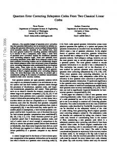
ˆ 11111 CZ(1,. . . ,4;5) X ˆ 11111 ), between qubits of the gate (X Grover state, for which two additional qubits are needed. ˆ 11111 = X ˆ ⊗X ˆ ⊗X ˆ ⊗X ˆ ⊗ X) ˆ The simplectic notation (X will be used to express the tensor product of Pauli operators (see Ref. 3, Preskill), and CU(i;k) means a control-U gate acting on the k-qubit depending on the i-qubit value. The total circuit [?] for the Grover algorithm appears in Fig. 3. Two calculations have been made with ε = γ = 0.001, 0.01 whose results are compared with the case in which there is no decoherence (ε = γ = 0). As can be appreciated in Fig. 4, even for a small search such as the present one (32 elements), the error effect quickly destroys the advantages of

F IGURE 3. Quantum Circuit implementing the Grover search algorithm for a data base with 25 terms. The oracle detecting the searched state (|X0 i =|11111i) is simulated by means of four Toffoli gates. Open circles represent |0i states.

the algorithm. Whereas for ε = γ = 0.001 the first maximum of the probability for the searched state reaches a value of 0.8, for ε = γ = 0.01 its value is only 0.2. Decoherence causes an attenuation of the Grover oscillations until the limit value of 1/32 is reached, in the long-time region.

7.

Quantum strategies for error control

Two great strategies for the error control can be implemented: passive methods, useful when we need a transmission of information over short distances. The most elementary are based on a complete isolation between the computer and its environment to minimise the noise. A second general method implies an active stabilisation (necessary in more complex processes) by means of some type of error detection and correction. Classic deteriorated information is still recoverable if some redundancy has been introduced. Unfortunately, it is not possible to use this redundancy in the quantum case, due to the impossibility of cloning unknown qubits. However, methods have been developed that allow us to control the qubit decoherence, thus solving the second problem settled in Sec. 4. Next we review some of the main strategies (Fig. 5). 1. Quantum error preventing codes (QEPC) These codes could be described as active methods in the sense that they prevent the occurrence of errors, although if these do take place they are incapable of correcting them. They are based on the quantum Zeno effect. 2. Quantum error avoiding codes (QEAC) These encode the information in states of certain subspaces that do not undergo decoherence, and are called decoherence free-subspaces (DFS). Error detection is not needed and they are useful with specific types of noise. 3. Quantum error correcting codes (QECC) This is an ˆ R), ˆ made up active strategy defined as the pair Q(E, ˆ ˆ of an encoding operation E and a recovery method R. They are methods capable of detecting and correcting quantum errors.

F IGURE 4. Evolution of the coefficient squared (probability) for the searched state (|11111i) versus time. Time means the number ˆ applied. Solid line represents the evolution of Grover gates (G) without error; dashed lines include error: • ε = γ = 0.001 and o ε = γ = 0.01.

F IGURE 5. Scheme of different strategies for error control.

Rev. Mex. F´ıs. E 52 (2) (2006) 218–243

INTRODUCTION TO ERROR CORRECTING CODES IN QUANTUM COMPUTERS

Notice that the corrected final system could still contain some errors, shown in Fig. 5 as a heavy line around the system (and a somewhat deformed ψ ) that differentiates it from the initial state. The QEPC are applied before the errors accumulate dangerously. On the other hand, the QEAC circumvent the problem of errors appearing. Even in this case, the final state can contain errors since the symmetries upon which these methods are based can only be approximate. Finally, the QECC are even applied after the appearance of errors. Actually, the above distinction among the different quantum codes or strategies is not as radical as it could seem. For instance a QECC applied very quickly could have the effect of a QEPC. Otherwise, some errors could not affect the encoded states of a QECC, so for these errors the code is functioning as a QEAC. In spite of that, the previous classification helps us to arrange the methods used to control the decoherence. Next we review each of the strategies, placing special emphasis on the well-developed QECC, although because the quantum circuits implementing them are expensive, they are giving way to other strategies which avoid errors.

8.

Quantum error preventing codes (QEPC)

These are codes preventing the appearance of errors, although if they do take place, these codes are incapable of correcting them. They are based on the quantum Zeno effect: measuring repeatedly on a system, this continuously collapses freezing its evolution and avoiding the errors [?]. The use of this effect to prevent errors was suggested initially by Zurek [?]. Let us consider a system described by the initial state vector |φ(0)i, representing a quantum register of length n. Suppose the system evolves unitarily under the Hamiltonian ˆ =H ˆ0 + H ˆ e (since there is no danger of confusion, we use H ˆ 0 dethe same notation as for a Hadamard rotation), where H ˆ e represents an error. Under scribes a perfect evolution and H these conditions, the state vector after a certain time δt can be expressed (with h/2π = 1) as: ˆ

|φ(δt)i =e−iHδt |φ(0)i =a(δt) |φ(0)i +b(δt) |ψ(0)i , (18) where |ψ(0)i is an state orthogonal to |φ(0)i. After a time δ t, the probability of obtaining the state |φ(0)i when measuring on |φ(δt)i is |a(δt)|2 , and its value can be expressed as ˆ hφ(0)|exp(−iHδt)|φ(0)i. The probability for short times δt is D D E E 2 ˆ ˆ )2 δt2 =1−(∆E)2 δt2 (19) |a(δt)| ≈ 1− (H− H The probability that we project the state |φ(δt)i on the subspace generated by {|ψ(0)i} (outside the subspace of interest generated by |φ(0)i) behaves like O(δt2 ). Sufficiently frequent measurements make the error probability as small as one wishes. This strategy is used in the stabilisation by the symmetrisation method that could be considered as an extension of the majority voted method to the quantum scale. Next we consider the formalism introduced in Ref. 13.

225

Let us suppose that each computation time step has the probability of producing a correct result (1-η) (with η constant); after N steps, the probability of success is (1-η)N ∼ exp(-ηN), decreasing exponentially with N. If we have a stabilisation method that diminishes the error by a factor 1/R per step, after N time steps, the probability of success will be exp(-ηN/R) which can be within a (1-δ) value, choosing R = ηN/-log(1-δ), having a polynomial dependence on N. Therefore, an exponential error growth (such as appears in the decoherence) can become stabilised by means of a method that reduces the error 1/R in each step. In this formalism, R is the redundancy introduced. The application of this stabilisation method is as follows. If we carry out the same computation in R copies of our quantum computer, they work independently and without errors, the total state of the R computers will be the tensor product: |Ψ(t)i = |φ(t)i(??) ⊗ . . . ⊗ |φ(t)i(R) ,

(20)

where all |φ(t)i(i) represents the same state, introducing a certain type of quantum redundancy. This state, in which there is no error, belongs to a symmetrical subspace of whole Hilbert space H⊗R . An error in a computation (or in all of them), would imply different vectors, so: |Ψ(t)e i = |φ(t)1 i ⊗ . . . ⊗ |φ(t)R i

(21)

Defining a symmetrical subspace HSIM ⊂ H⊗R as the smallest subspace of H⊗R containing the vectors of the form: R

⊗ |χi(i) ,

i=1

(22)

projecting the noisy |Ψ(t)e i state into HSIM would eliminate some of its errors. In summary, the stabilisation method eliminates the possible errors projecting a state of R copies of our computer on the HSIM subspace. The advantage of this process is that the dimension of H⊗R is 2R , whereas the one of HSIM is R+1, if the dimension of H is 2. The HSIM subspace has a dimension exponentially smaller than H⊗R . Nevertheless, not all the errors are eliminated, since in HSIM there are more vectors than those of the form |φi⊗. . . ⊗|φi. In spite of that, it can be demonstrated that the error decreases by a factor R in each symmetrisation.

9.

Quantum error avoiding codes (QEAC)

These are strategies that encode the information in states of certain subspaces that do not undergo decoherence, therefore they do not need to detect errors. These methods are useful with certain types of noise having some symmetry. The idea arose in a work of Palma [14] where they were called avoiding codes, later on to be called decoherence-free subspaces (DFS) [15]. A simple model will clarify the main idea.

Rev. Mex. F´ıs. E 52 (2) (2006) 218–243

226

P.J. SALAS-PERALTA

Let us suppose that single qubits undergo a decoherence, introducing a random phase angle φ independent of the system space coordinates: |0i → |0i and |1i → eiφ |1i

(23)

A qubit |qi = a|0i + b|1i put under this noise suffers a rapid loss of coherence. The decoherence effect on a subspace of dimension 4, made up of two qubits, is: |00i → |00i

|01i → eiφ |01i

|10i → eiφ |10i

|11i → ei2φ |11i

(24)

Since the states |01i and |10i acquire the same phase, if we use the encoding |0E i = |01i and |1E i = |10i, a general qubit encoded as |qE i = a|0E i + b|1E i evolves under the noise until the state eiφ {a|0E i + b|1E i}. The phase appearing has no importance and the subspace generated by {|01i, |10i} is a decoherence-free subspace. The fact that the phase φ does not depend on space coordinates causes the decoherence to be invariant under qubit permutations. The recognition of such types of symmetries is what allows the introduction the decoherence free subspaces in which the system evolution is purely unitary.

10. Quantum error correcting codes (QECC) ˆ R) ˆ made up of an A QECC can be defined as a pair Q(E, ˆ ˆ These are encoding operation E and a recovery method R. methods capable of detecting and correcting errors. Despite the impossibility of introducing redundancy as in the classic codes, it is feasible to disperse the quantum information embodied in the qubit, allowing its recovery after undergoing certain types of errors. Given a qubit |qi = a|0i + b|1i, its ˆ H⊗k → H⊗n from the Hilbert encoding is an application E: subspace of dimension k to a Hilbert space of a greater dimension n. The simplest case is to encode a single qubit (k = 1), where n is the number of qubits in the code states (registers). Formally, to maintain the number of qubits in the application, (n-1) initial qubits |0i are introduced, and the qubit |qi can be encoded as: ¯ n Eo ˆ (a |0i +b |1i) ⊗ ¯¯0⊗(n−1) E = |qE i =a |0E i +b |1E i , (25) ˆ is the encoding operation and the qubits |0E i and where E |1E i are called encoded. The application only chooses an encoding subspace or quantum code Q ⊂ H⊗n of dimension two. So, for the encoding to be useful, it must fulfil two conditions: a) The error subspaces must be distinguishable To identify the errors they must transform the encoded states of Q to states of mutually orthogonal subspaces in H⊗n .

b) Maintaining the coherence The correction process must conserve the qubit coherence. Inside each orthogonal subspace, the total state must be the tensor product of the qubit and the environment state. This behaviour allows the erroneous qubit to be recovered by means of a measurement that projects the total state into one of those subspaces (see Eq. 14). After measurement, the qubit is uncoupled from the environment, and once the subspace on which we have projected is detected, we will be able to correct the error. 10.1.

Quasi-classic error correcting codes

The simplest case in error correction consists of considering only bit-flip errors as in the classic case. Bit-flips attack the qubit |qi = a|0i + b|1i, transforming it into a|1i + b|0i. We must be able to detect the error without destructively measuring the qubit, otherwise we would destroy its coherence. Next we review the fundamental steps of the whole process. 10.1.1. Error model In addition to the aforementioned noise characteristics, we assume a symmetrical binary channel with an ε ( FW E to be fulfilled, ε < 0.5 is required (as in the classic case).

Fidelity = M in {hqE (0)| tre [| Ψ(t)i hΨ(t) |] |qE (0)i} . ∀|qE (0)i

(33)

Fidelity does not depend on the initial state considered, but only on the particular process, through |Ψ(t)i. The main objective of error correction is to maximise the fidelity. Considering only bit-flip errors, if we sent a qubit |q(0)i without encoding (or using error correction) the fidelity would be: ½ ¯ ¯2 ¾ ¯ ˆ |q(0)i¯¯ =1−ε (34) FW E = M in (1−ε)+ε ¯hq(0)| X ∀|q(0)i

Since the second term is positive and its minimum value corresponds to the case |q(0)i = |0i with zero value, the fidelity behaves as FW E ∼ 1-O(ε). Let us assume now that we encode the qubit |q(0)i with a quantum code Q = [[3,1,3]], that corrects one bit-flip error in any one of the three qubits in the register |qE (0)i. Supposing that the correction process is error free, all the errors affecting one qubit can be eliminated, which is reflected in the term 3ε(1-ε)2 of the (encoded) fidelity: © ª FE = M in (1 − ε)3 +3ε(1−ε)2 +positive terms (35)

10.3.

Error correcting codes for phase-flip errors

Phase-flip errors are typically quantum, although their correction is related to the bit-flip errors. They arise when the entanglement of the system with its environment gives rise to a phase decoherence. The general noise characteristics considered are the same as those of the previous case. In order to look for the appropriate encoding, we see that there is a close relationship between the bit-flip errors and those of phase-flip, through the form of the operators that produce them. The phase-flip errors can be ˆ H ˆX ˆ H, ˆ where H ˆ is a represented by Zˆ operators, but Z= Hadamard rotation. We use as codewords of the new Qf ˆ ⊗n {|0E i , |1E i}, where |0E i and |1E i are codewords code H of a code Qb correcting single bit-flip errors (and therefore with minimum distance 3). Encoding the qubit |qi provides ˆ ⊗n |0E i + bH ˆ ⊗n |1E i. If the channel introduces |qE i = aH ˆ a phase-flip error Ze in the qubit |qE i, we will have Zˆe |qE i = Zˆe

n

o ˆ ⊗n |0E i + bH ˆ ⊗n |1E i aH

∀|qE (0)i

and, applying the recovery operator ˆ= R

n

o n o ˆ ⊗n X(correction, ˆ ˆ (a) Sˆ H ˆ ⊗n = H ˆ ⊗n X(correction, ˆ ˆ (a)CN OT (q; a)H ˆ ⊗n , H a) M a)M

(36)

we obtain: on ³ ´o n o n ˆ ˆ (a)CNOT(q; a)H ˆ ⊗n ˆ ⊗n |0E i + bH ˆ ⊗n |1E i |00a i ˆ Zˆe |qE i = H ˆ ⊗n X(correction, a)M Zˆe aH R n o ˆ ˆ (a)CN OT (q; a) aX ˆ e |0E i + bX ˆ e |1E i |00a i ˆ ⊗n X(correction, a)M =H n o n o ˆ ˆ e |0E i + bX ˆ e |1E i |Se i = aH ˆ ⊗n |0E i + bH ˆ ⊗n |1E i |Se i ˆ ⊗n X(correction, =H a = Se ) aX

(37)

The CN OT (q; a) operation on the codewords |0E i and |1E i of Qb copy the bit-flip error information of the qubit q ˆ (a) represents the ancilla (control) onto the ancilla a (target), in accordance with the parity check matrix. The operator M ˆ measurement (whose result is the error syndrome |Se i) and the X(correction, a = Se ) represent the correction depending on ˆ ⊗n {|0E i , |1E i}. the ancilla measurement result. Finally, the encoded qubit is restored to the original encoded basis H If we take Qb = {|000i = |0E i, |111i = |1E i}, the new codewords of Qf are: ¯ E ˆ ⊗3 |000i = ¯¯0f = √1 ( |0i + |1i) √1 ( |0i + |1i) √1 ( |0i + |1i) H E 2 2 2 1 = √ { |000i + |001i + |010i + |100i + |011i + |101i + |110i + |111i} (38) 8 ¯ E ˆ ⊗3 |111i = ¯¯1f = √1 (|0i − |1i) √1 (|0i − |1i) √1 (|0i − |1i) H E 2 2 2 1 = √ {|000i − |001i − |010i − |100i + |011i + |101i + |110i − |111i} (39) 8

Rev. Mex. F´ıs. E 52 (2) (2006) 218–243

230

P.J. SALAS-PERALTA

With this code Qf

n o ˆ ⊗3 |000i , H ˆ ⊗3 |111i , the = H |qfE i

a|0fE i

b|1fE i.

qubit |qi = a|0i + b|1i is encoded as = + The two codewords of Qf are also orthonormal. Sending the qubit |qfE i through a noisy channel that introduces phase-flip errors, an entanglement with its environment occurs, similarly to that established in the previous code. The ˆ ijk for Zˆijk and their difference is replacing the operators X correlated environment states in Eq.(??). The set of correctable errors of Qf is:

sible: correcting quantum errors. The encoding was: ¯ © ®ª 1 ˆ |0i ⊗ ¯0⊗8 = |0E i = √ E (|000i + |111i) 2 2 × (|000i + |111i) (|000i + |111i) (41) ¯ ®ª 1 ˆ |1i ⊗ ¯0⊗8 = |1E i = √ E (|000i − |111i) 2 2 ©

× (|000i − |111i) (|000i − |111i) . (42)

So a qubit |qi=a|0i+b|1i is encoded into |q i=a|0 E E i+b|1E i. If there appears a bit-flip error in some CQf set of three qubits, it is possible to detect and correct it by means of an analogous method used with Q. If a phase-flip (40) error happens in one of these three sets, and we have some strategy to compare the sets, we will be able to detect and and the code for the phase-flip errors is Qf = [[3,1,3]]. Just correct them. Note that in Shor’s code, some errors such as like the Qb = Q code, there are errors that cannot be corrected, Zˆ110 , Zˆ101 or Zˆ011 , even though they do not produce orthogbut their weight is greater than those that can be corrected and onal states, are equivalent (equal) and correctable. These the encoded fidelity behaves like 1-O(ε2 ). codes are called degenerated. The syndrome measurement circuit and qubit correction Almost simultaneously Steane (1996) introduced a implementing Sˆ is analogous to the one in the previous case method for transforming certain types of classic codes into (Fig. 7), with the difference that the encoding is carried out in quantum ones. The idea that guided him was that bit-flip erthe base {|0fE i, |1fE i}, and three Hadamard gates must appear rors could be corrected with a code of a classic type, and the just before and after the error correction. phase-flip errors were equivalent to bit-flips if a Hadamard rotation were previously made. When rotating the codewords, it had to make sure that they did not leave some code 10.4. Phase and bit-flip error correcting codes of a suitable distance. Steane encoded two qubits |0i and |1i starting with The correction power of the previous codes is limited. The a classic Hamming code C = [7,4,3] containing its dual code Qb = [[3,1,3]] uses qubit redundancy to correct a single C⊥ = [7,3,4] (even subcode, since it contains only the bit-flip error; the Qf = [[3,1,3]] uses sign redundancy to corcodewords of even weight). The basis of the quanrect a single phase-flip error. Nevertheless, we must find a tum code include two entangled states obtained from single quantum code capable of correcting both types of erthe classic codewords of each coset of C relative to rors. Historically it was Shor [17] who in 1995 introduced C⊥ : C⊥ ⊕ (0000000) = C⊥ = {codewords of C with even weight}, the first code that did what for some time was thought imposand the C⊥ ⊕ (1111111) = {codewords of C with odd weight} (see Fig. 8). The quantum codewords are: ½ ¾ ¯ ⊥® 1 |0000000i + |0001111i + |0110011i + |0111100i ¯ |0E i = C = √ |1010101i + |1011010i + |1100110i + |1101001i 8 ½ ¾ ¯ ⊥ ® 1 |1111111i + |1110000i + |1001100i + |1000011i ¯ |1E i = C ⊕ (1111111) = √ (43) |0101010i + |0100101i + |0011001i + |0010110i 8 n = Iˆ ⊗ Iˆ ⊗ Iˆ ≡ Zˆ000 , Iˆ ⊗ Iˆ ⊗ Zˆ ≡ Zˆ001 , o Iˆ ⊗ Zˆ ⊗ Iˆ ≡ Zˆ010 , Zˆ ⊗ Iˆ ⊗ Iˆ ≡ Zˆ100

The vector space generated by the (encoded) computation basis F = {|0E i, |1E i} corresponds to a quantum code Q (analogous to Qb ) correcting one bit-flip. In addition to the F basis, we can use other bases, for example the dual (encoded) ˆ ⊗7 |0E i, H ˆ ⊗7 |1E i}: basis P = {H ˆ ⊗7 |0E i = √1 {|0E i + |1E i} H 2 ˆ ⊗7 |1E i = √1 {|0E i − |1E i} H 2

consisting of two entangled and orthonormal states involving codewords of the [7,4,3] classic code that can correct one bit-flip error. 10.4.1. Detection and error correction

(44)

Since the quantum encoding uses linear combinations of classic codewords (in C) of distance 3, it is possible to detect sinˆ e error (the error is gle bit-flip errors. The appearance of an X applied to the qubits where the vector e ∈ GF(??)7 has 1’s), ˆ e {|0E i, |1E i}, moves the codewords {|0E i, |1E i} towards X

Rev. Mex. F´ıs. E 52 (2) (2006) 218–243

INTRODUCTION TO ERROR CORRECTING CODES IN QUANTUM COMPUTERS

231

both in the same coset of C, maintaining coherent superpositions. In order to measure the syndrome, an ancilla with three qubits (|000a i) is used into which the syndrome is copied by means of CNOT gates placed according to the parity check matrix of C=[7,4,3]: 

H[7,4,3]

1 = 0 0

0 1 0

1 1 0

0 0 1

1 0 1

0 1 1

 1 1  1

(45)

The measurement of the ancilla qubits provides the syndrome bits in accordance with which NOT gates are applied ˆ (X(correction, a)) where necessary. The bit-flip errors proˆ e |qE i = |qE ⊕ ei, and the correction can be duce the effect X outlined as: n o n o ˆ X ˆ e |qE i = X(correction, ˆ ˆ (a)CN OT (q; a) R a)M × |qE ⊕ ei |000a i ˆ → X(correction, a = Se ) |qE ⊕ ei |Se i = |qE i |Se i

(46)

A phase-flip error transforms the qubit into Zˆe |qE i. Its detection involves a seven-qubit Hadamard rotation. By ˆ Zˆe = X ˆeH ˆ condition, we transform phasevirtue of the H flip errors in basis F into bit-flip errors in the P basis. The relationship between both bases can be understood easily. A phase-flip error in the computation basis F (|0i → |0i and |1i → −|1i) corresponds to a bit-flip error in the dual basis P ˆ ˆ ˆ ˆ (H|0i → H|1i and H|1i → H|0i). As the P basis involves C codewords of distance 3, it is possible to make a correction for bit-flips using a three-qubit ancilla state. We apply a set of CN OT (q; a) gates to obtain the error syndrome and correct ˆ with X(correction, a = Se ) gates. To conclude, we rotate back the qubit state to leave it in the original computation basis. The complete correction circuit is shown in Fig. 9.

F IGURE 9. Quantum circuit implementing the syndrome extraction and qubit correction when it is encoded (|qE i) by means of Steane’s [[7,1,3]] quantum code. In order to measure the syndrome for he bit-flip and phase-flip errors, six ancillas in the initial state |0a i are used.

The syndrome (S1 , S2 , S3 ) describes bit-flip errors, whereas (S4 , S5 , S6 ) corresponds to the phase-flip errors. Correcting both, it is also done for the Yˆe errors, because ˆ e . We conclude that the Steane code is [[7,1,3]] Yˆe = Zˆe X ˆ Yˆ and Zˆ error. and corrects any X, 10.4.2.

CSS codes

The construction method of the Steane [[7,1,3]] code can be generalised to obtain other codes. We now describe a family of codes called CSS, whose design is based on the theory of classic linear codes. Discovered by Calderbank, Shor [18] and Steane [19], with the Steane’s code being a particular case, the method is based on the theorem of the dual code. Theorem of the dual code: By rotating Hadamard, a quantum state obtained as the linear combination of all the codewords of a linear classic code C = [n,k,d], we get a state which is the linear combination of all the codewords of its dual C⊥ (linear) code: X X 1 ˆ ⊗n √1 H |ii = √ |xi. 2k i∈C 2n−k x∈C ⊥

F IGURE 8. Relationship between the GF(??)7 = {0, 1}⊗7 vector space and the subspaces conforming the [7,4,3] Hamming code and its dual.

(47)

The CSS construction is as follows. Consider two classic linear codes: C1 = [n,k1 ,d1 ], whose parity check matrix is H1 [(n-k1 )×n], and C2 , with parity check matrix H2 [(n-k2 )×n], are such that C2 (subcode) ⊆ C1 . Then k2 < k1 and the parity check matrix of H2 contains (n-k1 ) rows of H1 and some other (k1 -k2 ) linearly independent rows, assuring C2 ⊆ C1 . The subcode C2 defines an equivalence relationship < in C1 : ∀u, v ∈C1 , u < v ⇔ u-v ∈ C2 , or, which is the same, u < v ⇔ if ∃ w∈C2 | u = v + w. The equivalence classes are cosets of C1 relative to C2 (elements of the factor group C1 /C2 ). The number of cosets is 2k1 /2k2 = 2k1 −k2 . Let us transform the classic codewords of coset C2 ⊕a (a∈C1 ) into quantum states and construct an

Rev. Mex. F´ıs. E 52 (2) (2006) 218–243

232

P.J. SALAS-PERALTA

entangled state of the type: |C2 ⊕ ai = √

10.4.3. Stabiliser codes [21] 1

X

2k 2

i∈C2

|i ⊕ ai.

(48)

The set of these states forms an orthonormal base of a subspace of dimension 2(k1 −k2 ) of the Hilbert space H⊗n (see Fig. 10). The states |C2 ⊕ ai are created by the linear combination of distance d2 codewords of a C2 code, so it will be capable of correcting t2 = b(d2 − 1)/2c bit-flip errors. In addition, as the syndrome of all the codewords depends solely on the error, the syndrome extraction will maintain the qubit coherence. In general we can provide the following Definition: Given two linear classic codes C1 = [n,k1 ,d1 ] ⊥ and C2 = [n,k2 ,d2 ] (its dual being C⊥ 2 = [n, n-k2 , d2 ]) so that C2 (subcode) ⊆ C1 , the subspace generated by the encoded base {|C2 ⊕ ai, a∈C1 } is a quantum CSS code Q(C1 , C2 ) = [n,k1 -k2 ,D] of dimension 2(k1 −k2 ) and distance D ≥ Min{d1 , d⊥ 2 }. In order to construct quantum codes with this method, it is sufficient to look for classic codes contained in its dual (or vice versa). Given a classic code C, if C ⊂ C⊥ is fulfilled, it is called weakly self-dual. An example of weakly selfdual and self-dual linear binary codes (C = C⊥ ) that cover a large interval of distances and code rate (k/n) is the family of Reed-Muller codes (RM) [?]. Starting with self-dual RM codes, quantum codes of dimension one can be constructed as [[n,0,d]]. From the [[8,4,4]] [[32,16,8]] and [[128,64,16]] RM codes, we obtain [[8,0,4]], [[32,0,8]] and [[128,0,16]] respectively. In order to obtain codes with dimension two, the self-dual RM codes can be punctured, their dual code being an even subcode. Puncturing (deleting coordinates) the [[8,4,4]], we get [[7,4,3]], which contains the even subcode [[7,3,4]], providing the well-known [[7,1,3]] Steane quantum code. From the other weakly self-dual RM codes, the [[31,1,7]] and [[127,1,15]] are derived, correcting errors of weight 3 and 7 respectively. From RM codes of greater dimension such as [[64,42,8]] (whose dual is [[64,22,16]]), other quantum codes can be obtained such as [[64,20,8]].

Quantum codes are certain vector subspaces of H⊗n . A way to specify them is as the common eigenspaces of a set of commuting operators, forming itself an abelian sub-group (called stabiliser group SQ ) of the Pauli group. The Pauli group Gn is made up of the operators { ± 1} × {Aˆ{i1 ,i2 ,...,in } = Aˆ1i1 ⊗ Aˆ2i2 ⊗ . . . ⊗ Aˆnin }. In the case of the repetition code [[3,1,3]], we have a Hilbert space of dimension 23 . If we want to specify the code as a subspace of dimension 2, we can use the eigenspace common to two operators. Foroexample, the n ˆ ˆ common eigenspace of the set Z110 , Z101 is the code Q = {|000i, |111i} ≡[[3,1,3]], which is where an encoded qubit resides when it does not have errors. The set can be transformed into a group SQ if the product of its operators is included. This SQ group is abelian and is called stabiliser, because its operators fix the codewords of the quantum code ˆ factor group. Q. Actually, SQ is a subgroup of the Gn /{±I} ˆ is the centraliser of Gn , so that we do not care The {±I} about the global operator phase, and SQ is abelian. D SQ can be E specified completely by its generators SQ = Zˆ110 , Zˆ101 (the notation h. . .i is used to specify the group generators.). If an encoded qubit |qE i undergoes an error ˆ v , its state becomes X ˆ v |qE i, and is fixed by X D E ˆ ˆ ˆ ˆ ˆ ˆ ˆ v because: Xv SQ Xv = Xv Z110 Xv , Xv Zˆ101 X ˆ v Zˆu X ˆ v (X ˆ v |qE i) = X ˆ v Zˆu |qE i X ˆ v |qE i (u = 110, 101) =X

(49)

ˆ v |qE i ∈ X ˆ v Q. The syndrome is determined by the exand X istence of an operator in SQ anticommuting with the error ˆ v . If X ˆv = X ˆ 100 , operator X o n ˆ 100 , Zˆu X n o ˆ 100 , Zˆ100 Zˆ(100)⊕u =0 (u=110, 101) (50) = X ˆ 100 commute with Zˆ010 and Zˆ001 : since X ³ ´ ˆ 100 |qE i =Zˆ100 X ˆ 100 Zˆ001 |qE i =−X ˆ 100 Zˆ101 |qE i Zˆ101 X ˆ 100 |qE i = (−1)a X ˆ 100 |qE i (51) = −X

³ ´ ˆ 100 |qE i = −X ˆ 100 Zˆ110 |qE i Zˆ110 X

ˆ 100 |qE i = (−1)b X ˆ 100 |qE i (52) = −X

F IGURE 10. Construction process of a CSS code from the code C2 ⊆ C1 . Each box represents a coset with a different syndrome depending on the displacement vector.

ˆ 100 error is (a,b) = (1,1). An error The syndrome of the X operator anticommuting with an operator in SQ changes the eigenvalue of the state from +1 to –1. Fig. 11 shows the single bit-flip error syndromes and their orthogonal subspaces.

Rev. Mex. F´ıs. E 52 (2) (2006) 218–243

INTRODUCTION TO ERROR CORRECTING CODES IN QUANTUM COMPUTERS

F IGURE 11. Relationship of the different subspaces from the repetition code that corrects one bit-flip. The pairs in parenthesis indicate the error syndrome in each subspace. For the code, the syndrome is (a,b) = (0,0).

233

In the case of the Steane code, the stabiliser is generated by 6 operators (obtained by replacing the 1’s in the rows of ˆ or Zˆ operators), whose common H[7,4,3] , Eq. (45), by X eigenspace, with eigenvalue +1, makes up the code [[7,1,3]]. Shor’s [[9,1,3]] code can be described by means of a stabiliser with 8 generators. CSS codes are stabilisers; nevertheless these latter contain other codes that are not CSS. For example, the perfect quantum code [[5,1,3]] [22](saturates the quantum Hamming bound 2(1 + 3n) ≤ 2n for codes with d=3, [?], analogous to classic equation 5), is not a CSS code although it is a stabiliser. Given that the errors change the eigenvalue of the SQ generators, the correction circuit construction can be described in a more general way as the collective measurement of these operators. The measurement of operators is a fundamental element in error correction. The objective is to project the qubit state on an eigenstate of SQ , at the same time as we keep an indicator from the eigenvalue in some quantum register. Let us suppose that we have a hermitian operator (such as an observable) and unitary (which can also represent a time ˆ , having the ±1 eigenvalues. In order to measure evolution) U ˆ U , we must make a projection of the qubit on one of its two eigenspaces. The circuit implementing the measurement appears in Fig. 12. The initial state of the qubit is |qi i and an ancilla in the |0i state is used. Its joint evolution is:

ˆ. F IGURE 12. Measurement circuit for the hermitian operator U The gate connecting both qubits is a control-U. ˆ H ˆ 1 I⊗ |qi i |0a i = {a |0i + b |1i} |0a i −→ {a |0i + b |1i} √ {|0a i + |1a i} 2 n o CU (2;1) 1 ˆ |0i) |1a i + b |1i |0a i + b(U ˆ |1i) |1a i −→ √ a |0i |0a i + a(U 2 nh i h i o ˆ H ˆ 1 I⊗ ˆ |0i + bU ˆ |1i ⊗ |0a i + a |0i + b |1i − aU ˆ |0i − bU ˆ |1i ⊗ |1a i −→ a |0i + b |1i + aU 2

The CU(2;1) means a control-U gate acting on the qubit 1 (target) depending on the qubit 2 value (control). The projectors on the eigenspaces with eigenvalues ±1 are ˆ )/2. Measuring the ancilla qubit of the previPˆ± = (Iˆ ± U ous evolution, if we obtain the state |0a i, we will have projected according to Pˆ+ ; and if the result is |1a i, the projection will correspond to Pˆ− . Note that the qubits used can be either non-encoded or encoded. Using this construction, we obtain the circuit shown in Fig. 13. To determine the syndrome, the operators Zˆ110 and Zˆ101 are measured by means of two ancilla qubits initially in state |00a i. Bearing in mind ˆX ˆH ˆ (Fig. 14), it is easy to obtain the the equivalence Zˆ = H circuit as it appears in Fig. 7.

(53)

F IGURE 13. Quantum circuit measuring the generators Zˆ110 and Zˆ101 of the [[3,1,3]] code. Gates M provide the error syndrome.

F IGURE 14. Equivalence of circuits used in the syndrome extraction. Rev. Mex. F´ıs. E 52 (2) (2006) 218–243

234

P.J. SALAS-PERALTA

10.4.4. Codes on GF(??) It is possible to relate the stabiliser quantum codes and the classic codes in GF (4)[24], establishing an isomorphism between the elements of the stabiliser and those of a subcode of GF(??)n that is selforthogonal with respect to a certain symplectic product. This is the case in the [[5,1,3]] code that comes from a Hamming code in GF(??). This connection with the classic codes has allowed the well-known constructions of these codes to be used to obtain a great number of new quantum codes with a distance greater than 3, correcting more than one error. In the same way, stabiliser codes can be generalized to nonbinary alphabets over finite fields [25]. 10.5. Quantum operation formalism applied to QECC The fundamental pieces of quantum error correction are quantum states to be protected and noise. There are several ways to point out the theory [26]. Until now, we have used state vectors or kets emphasizing the environmental effect on the system studied as givin rise to the errors. Experimentally it is not possible to know environment states, so a formalism based on the concept of quantum operations (or superoperators, see Knill and Laflamme in Ref. 3) [?] will be more general and powerful to treat the evolution of open systems such as quantum computers. In general, quantum states are described by means of the density operator ρˆ (or density matrix, if a basis set is chosen), and its time evolution by the quantum operation E defined as a map ρˆ → E(ˆ ρ), which has the following properties: 1.- E is a convex-linear map in the density operator set, fulfilling: Ã ! X X E pi ρˆi = pi E(ˆ ρi ), (54) i

i

{pi } being the probability set for the {ˆ ρi } states. ˆ S ) is more than 2.- E is a completely positive map. E(O ˆ S of the a positive operator for any positive operator O system S. Consider all possible extensions T of S to the combined system TS; then E is completely positive in ˆ T S ) is positive for any positive operator S if (IT ⊗E)(O ˆ OT S of TS. 3.- The value 0 ≤ tr[E(ˆ ρ)] ≤ 1 is the probability that the process represented by E will occur when ρˆ is its initial density operator. Analogous to the one-qubit evolution of Eq. (11), the evolution of a system such as an n-qubit register |q1 ,. . . ,qn i in contact with the environment (in the initial state |ei) can be expressed as: ˆ {|q1 , . . . , qn i ⊗ |ei} U ´ X³ ˆi |q1 , . . . , qn i . (55) |µ(t)i i ⊗ B =

An orthonormal environment basis set {|µi i} has been ˆi could be (in general) linear comused. Now the operators B binations of (tensor product) Pauli operators [see Eq. (16)] because of the basis change from {|ei i} to {|µj i}. The evolution operator eliminates the possible initial factorization between the state of the register and the environment. Suppose the initial state is characterized by the tensor product of the density operator for the system and the environment: ρˆ(0)s ⊗ ρˆ(0)e . The whole evolution can be written as ρˆs (0) ⊗ ρˆe (0)

ˆ Evolution:U

−→

ˆ [ˆ ˆ+ ρˆ(t) = U ρs (0) ⊗ ρˆe (0)] U → ρˆrs (t) = tre {ˆ ρ(t) } , (56)

ρˆ(t) being the density operator of the {system + environment} at time t, ρˆrs (t) the reduced density operator (or matrix) of the system obtained by taking the partial trace with the environment states. Carrying out the calculation: X ˆ [ˆ ˆ + |µi i ρˆrs (t) = tre {ˆ ρ(t)} = hµi | U ρs (0) ⊗ |ei he|] U i

=

X

ˆ |ei ρs (0) he| U ˆ + |µi i hµi | U

i

=

X

ˆi ρˆs (0)B ˆ +, B i

(57)

i

ˆi = hµi | U ˆ |ei are operators acting on the Hilbert where B space of the system. Using the definition, it is not difficult to show the normalization condition X ˆ +B ˆ i = Is B i i

(identity for the system). The map ρˆs (0)αE(ˆ ρs (0)) = ρˆrs =

X

ˆi ρˆs (0)B ˆ+ B i

(58)

i

defines a quantum operation representing the density operator evolution of the system alone. All the environment effect ˆi , called interaction operators. The breaking is hidden in B ˆi is called the operator-sum repdown of ρˆrs in terms of B resentation or Kraus representation. Note that this represenˆi is not unique because it is environment tation in terms of B basis-dependent. The depolarizing error model applied to a qubit q and shown in Eq. (15) can be described now by means of the following interaction operators: r √ ε ˆ ˆ ˆ ˆ B1 = 1 − εA1 Bi = Ai with i = 2, 3, 4 (59) 3 describing the evolution of a qubit density operator: ρˆq (0) → E(ˆ ρq (0)) = ρˆqr (t) = (1 − ε)ˆ ρq (0)

i

Rev. Mex. F´ıs. E 52 (2) (2006) 218–243

4

+

εX ˆ Ai ρˆq (0)Aˆ+ i . 3 i=2

(60)

235 o ˆi , have {da } as eigenvalues. For each da 6= 0 (if da = 0, B

INTRODUCTION TO ERROR CORRECTING CODES IN QUANTUM COMPUTERS

Redefining the parameter ε = 3p/4, the reduced density matrix is: Iˆ E ( ρˆq (0)) = ρˆqr (t) = p + (1 − p)ˆ ρq (0). 2

(61)

Its evolution is now very transparent, showing two contributions: the untouched qubit with probability (1-p), and a ˆ with probability p. completely mixed state I/2 The correction process can be seen as the search for the inverse quantum operation E −1 . Although the E −1 in the whole Hilbert space (H⊗n ) only exists in the case of a unitary operator, it is possible to invert it, taking the restriction to some special subspaces Q ⊂ H⊗n . The quantum recovery operation R fulfils the condition: ∀ρ defined in Q, R(E(ρ)) ∝ ρ

(62)

The recovery R reverses the errors represented by E, mapping them into an operator proportional to the identity [Eq. (62)]. The notion of detectable errors has been explicitly introduced by Knill and Laflamme [3], and can be established ˆ is detectable by the quantum code Q if and thus: an error B only if ˆ |vi = 0 (63) ∀ |ui , |vi ∈ Q fulfilling hu| vi = 0 ⇒ hu| B ˆ transforms the Q-codewords, keeping their The error B orthogonality and making it possible to differentiate them. ˆ is detectable by Q if and only if the Alternatively, an error B ˆ ˆ ˆ condition PQ B PQ =αB PˆQ is satisfied for a complex conˆ PˆQ being the projector stant αB depending on the error B, operator in Q. Without going into a full demonstration (see details in Nielsen and Chuang [3] and [27]), imagine the condition is fulfilled ∀|φ1,2 i ∈ H⊗n , and PˆQ |φ1,2 i = |u1,2 i ∈ Q.

If

hu1 | u2 i = 0,

the condition means ˆ PˆQ |φ2 i = hu1 | B ˆ |u2 i = αB hu1 | u2 i = 0. hφ1 | PˆQ B ˆi } is called correctable Consequently, a set of errors CQ = {B ˆ ˆ+ by the code Q if and only if the set CQ C+ Q = {Bi Bk } is detectable. Eqs. (32) are an example of that fact. ˆi B ˆ + PˆQ = αik PˆQ , it is From the general condition PˆQ B k possible to obtain the recovery quantum operation R. As a quantum n o operation, it is characterized by means of the set ˆ i defining the map: R ρˆ → R(ˆ ρ) =

X

ˆ i ρˆR ˆ+. R i

(64)

i

ˆi B ˆ +, The matrix αik depends only on the error operator B k + ˆ ˆ and its elements are αik = hu| Bi Bk |ui, |ui ∈ Q. Because it is it can be diagonalized, and the new set of errors n hermitian o ˆ Ni , obtained as the appropriate linear combinations of

n

ˆa |ui = 0, ∀|ui ∈ Q), a recovery quantum operation can be N defined as:   X 1 ˆa+ , ˆa = √  |ui hu| N (65) R da |ui∈Q ³ ´ √ ˆb = da δab IˆQ for the states ˆa N fulfilling the condition R ˆ a corrects N ˆa in Q, and R corrects any in the code Q. Then R ˆ linear combination of Na errors. Notice that, strictly speaking, in order to have a quantum recovery operation R, it has to be extended to the whole Hilbert space (for mathematical details see Preskill [?]), which can be split as µ ¶ ˆa Q ⊕ Q⊥ , H ⊗n = ⊕ N a

where Q⊥ is the orthogonal complement of the code Q which ˆa . is not reached acting on the code with the operators N In order to implement the recovery quantum operation, ˆ a can be written as: the operators R   X 1 ˆa = √  ˆa+ R |ui hu| N da |ui∈Q   X ˆa+ N ˆa+ PˆaQ . ˆa |ui hu| N ˆa+  = N =√  N da |ui∈Q

(66)

The operator PˆaQ projects onto the subspace ˆ Na Q ⊂ H ⊗n . Its implementation involves the projection ˆa Q according to PˆaQ , identifyof the corrupted state onto N ˆ ing the subspace Na Q characterized by the index a, and then ˆa+ . To carry out the recovery applying the inverse operator N process, an ancilla system is introduced, characterized by the Hilbert space HA and with a set of standard orthogonal states {|ar i}. Now we shall work within the subspace µ ¶ ˆ ⊕ Na Q ⊗ HA . a

The first step is to apply the unitary operator Vˆ (the |a0 i state is the initial ancilla state): X PˆaQ ⊗ |aSa i ha0 |. (67) Vˆ = a

The operator Vˆ is a generalisation of the standard ˆa Q ⊗ |aS i. The controlled-operation and will project onto N a ˆa ancilla state carries the syndrome information Sa of the N error. Measuring the ancilla in the standard basis we obtain ˆa+ , the the state |aSa i and, finally, applying the operator N error is reversed. This general process can be recognized in what was done in Fig. 7 (Sec. 10.1.7) and 9 (Sec. 10.4.1) for the three-qubit repetition code and Steane code, respectively.

Rev. Mex. F´ıs. E 52 (2) (2006) 218–243

236

P.J. SALAS-PERALTA

ˆ error propagation from the image qubit F IGURE 15. Phase-flip (Z) to the control qubit in the case of a CNOT gate connecting both qubits.

F IGURE 16. Forward bit-flip and backwards phase-flip error propagation, due to the application of a CNOT gate.

of the algorithm. The error correcting codes are the first step to reaching it, the second is the use of fault-tolerance techniques [?]. To implement a quantum gate, we could decode the quantum state, carry out the gate, and encode the state again. This process is not advantageous since, during the period of time in which the gate is put into operation, the information is unprotected. The fundamental idea of fault-tolerance is to use an encoded logic: applying the encoded quantum gates to encoded qubits [?], without a previous decoding. Nevertheless, the encoded logic, by itself, is not sufficient to ensure its tolerance to failures, and we will have to consider two additional aspects. In the first place, the application of encoded gates to encoded qubits can disperse the errors to other qubits within the same register as well as to other registers, until they become uncorrectable. Secondly, the error correction processes are also quantum computations, which is why they can introduce new errors. We will have to make an appropriate design of encoded gates and error correction circuits to control error dispersion and accumulation. After reaching these objectives, we shall make periodic encoded corrections to the qubits. 10.6.1. Error propagation

F IGURE 17. Encoded CNOT gate in the [[3,1,3]] code. The lefthand piece shows a perfect transversal CNOT gate performance when the control and target registers are |111i. On the right-hand side, a bit-flip error corrupts the third qubit of the control register, and is dispersed to the third qubit of the target register.

F IGURE 18. Dispersion of phase-flip errors in the measurement of one bit of syndrome S. On the left, a phase-flip error propagates from an ancilla qubit until the three qubits of the upper register. This error cannot be corrected. On the right there is an equivalent transversal version. A phase-flip error in the ancilla has been propagated exclusively to one qubit of the upper register. In this case the error could be correctable in later time steps.

10.6. Fault tolerance in QECC The final mission of the decoherence control in quantum computers is a static stabilisation of the information when it is transmitted or stays in the memory, as well as a dynamic stabilization of it. We need to process the information dynamically, applying gates without an excessive accumulation of errors, during the time sufficient to complete the execution

One of the frequent types of gates in the computation and error correction are the control-M (M = NOT, Z). Let us see how the CNOT gate propagates the errors. A bit-flip error in the control qubit of a gate CNOT, propagates forward towards the target qubit. In addition to this spread (of a classic type), a phase-flip error propagates backwards, from the target qubit to the control qubit. Let us suppose we have a CNOT gate whose control qubit is |qi = a|0i + b|1i and a phase-flip error occurs in the target qubit (|0i + |1i in Fig. 15). The ˆ propagates from the target to |qi. The phase-flip error (Z) bit-flip and phase-flip error propagation is shown in Fig. 16. Similar situations arise in gates involving several qubits, such as the Toffoli gate. If we use a code allowing a single error to be corrected in each quantum register, we define a faulttolerant procedure as one with the property that if an error occurs in one of its components, it causes (at most) one error in each register. The uncorrectable errors (for example in two qubits) take place with a probability O(ε2 ), ε being the probability per qubit that some time step or gate introduces an error. This definition can be generalized to codes that correct t errors, just by demanding that no more than t errors are introduced in each register after the procedure execution. In the case that single qubits of the same register are related by a CNOT gate, the dispersion of errors could be fatal. Some gates exist, depending on the code, which can be implemented by means of a transversal logic, which ensures its fault-tolerance. For example a CNOT gate can be transversally implemented in a [[3,1,3]] code, as shown in Fig. 17. A bit-flip error appearing in the third qubit of the control register propagates solely (following the arrow) to the third qubit of the target register. The CNOT gate is implemented

Rev. Mex. F´ıs. E 52 (2) (2006) 218–243

INTRODUCTION TO ERROR CORRECTING CODES IN QUANTUM COMPUTERS

transversally, by means of a procedure in which each qubit of the control register is connected to a single qubit of the target register. A transversally applied gate assures that it is fault-tolerant. An error in each register can be corrected in a later error correction step, thus avoiding its accumulation. The error probability that two uncorrectable errors occur in the control register (which would induce two errors in target qubit) behaves like O(ε2 ). Some gates cannot be implemented in a transversal form, as would be the situation for the Hadamard rotations in [[3,1,3]], and we should design more complex circuits that could involve qubit measurements. 10.6.2.

Fault-tolerant error-correcting circuits

Quantum error correcting codes imply encoding, syndrome measurement, and qubit correction processes using ancilla qubits, and adding new time steps and gates. In this situation, the errors become more probable, with new routes appearing in the error spreading. For the QECC to be useful, it is necessary for their implementation to be sufficiently robust, preventing more errors being introduced into them than they try to eliminate, as well as being sufficiently fast. Let us suppose that we use a QECC, and the probability that a register has an error is O(ε), arising from evolution or gate errors. The definition of a fault-tolerant error-correction circuit reflects the intuitive idea that it must correct more errors than are introduced by it. A quantum circuit (of a code with distance 3) is considered fault-tolerant if the probability of a register having an uncorrectable error after its execution behaves like O(ε2 ). In general, a quantum circuit correcting t errors is fault-tolerant if the probability of uncorrectable errors is O(εt+1 ). The tolerance to failures tries to avoid all ways in which such possibilities can take place. One of the most important steps in the correction processes is destructive and non-destructive measurements. These are used in the encoding, syndrome determination and ancilla synthesis (employed not only in error corrections, but in the implementation of encoded fault-tolerant gates); this is why its fault-tolerant accomplishment is of fundamental importance. Concerning codes with distance three, to get a fault-tolerant encoded measurement process, two conditions must be met: a) An error in any time step of the measurement process must produce one error in each register, and b) If an error occurs during the measurement process, the probability that the result of the measurement is incorrect must be O(ε2 ). The motivation of the first condition is that an error in a register is tolerable by the code and can be corrected in a later time step, whereas the second reflects the fact that the measurement results could be used to correct one or several qubits within a register. If the error probability in a measurement behaves like O(ε), the subsequent error correction using this result could introduce several errors into the same register with O(ε) probability, with them being uncorrectable.

237

The destructive measurement produces the collapse of the measured state. This is the case in the final ancilla measurement for obtaining the error syndrome. If the error probability is O(ε) in each qubit, and these are not correlated, the probability of an uncorrectable error taking place (two or more errors in the register) is O(ε2 ). So the destructive measurements are fault-tolerant. As well as the destructive measurements, we can measure hermitian operators non-destructively, such as the stabiliser generators, as we have already seen in Fig. 12. The syndrome copied into the ancilla, is found by measuring this last one destructively. Nevertheless a single ancilla state is not suitable for extracting the syndrome because the circuit could spread the errors in an uncorrectable way. As an example, let us look at a piece (Fig. 18) of the correction circuit shown in Fig. 9 (measurement of the syndrome S1 ). A phase-flip error in the ancilla qubit (we suppose in the state |1a i) used as the target of several CNOT gates is propagated to three qubits of the upper register. If the phase-flip error probability is O(ε), the propagation has introduced three errors affecting the upper register with the same probability, these being uncorrectable in later corrections (left-hand side in Fig. 18). This behaviour appears because the same ancilla qubit is the target of all the CNOT gates. We can solve the problem, by replacing the ancilla qubit by four, so that if there is an error in one of these single qubits, they propagate to a single qubit in the control register (the right-hand side of Fig. 18). Nevertheless this operation does not completely solve the problem. Let us see why in the following example. Suppose we use the Steane [[7,1,3]] code to get |0E i and |1E i, and a bit-flip error occurs in the seventh qubit, repˆ7 ≡ X ˆ e (e = (0000001)). To obtain one bit resented by X of syndrome (for example, measuring the Zˆ0001111 generator shown in Fig. 18), we use an ancilla state |0000a i, and four CNOT gates are applied involving four qubits of the encoded control register and four ancilla target qubits. The process would be as follows: ˆ 7 {a |0E i + b |1E i} |0000a i X = [a {|0000001i + . . .} four CNOT gates +b {|1111110i + . . .}] |0000a i −→ ³ ´ ³ ´ ˆ 7 |0E i |0001a i + b X ˆ 7 |1E i |1110a i (68) →a X Measuring the ancilla destructively, we will find two states |0001a i or |1110a i bringing about a collapse of the ˆ 7 |0E i or to X ˆ 7 |1E i, with probabilities |a|2 whole state to X 2 and |b| respectively. The initial qubit coherence has been destroyed, with certain information about it having been acquired. To cope with the problem, we need to synthesize special ancilla states and design appropriate recovery circuits. 10.6.3.

Ancilla states

Ancilla states are involved in syndrome measurement as well as intermediate states in fault-tolerant encoding and gates;

Rev. Mex. F´ıs. E 52 (2) (2006) 218–243

238

P.J. SALAS-PERALTA

therefore, the design of the ancillas is an important aspect in the fault-tolerant computation. In QECC, we require an ancilla state to copy the error syndrome onto it and one that we can measure destructively without losing the qubit coherence, and without introducing too many new errors. The syndrome measurement does not have to reveal anything about the state of the information qubit. DiVincenzo and Shor propose using a special ancilla state |aShor i synthesized from the Schr¨odinger cat-state (|0000i+|1111i), and Hadamard-rotating all qubits to obtain an entangled state of equal-weighted, even-parity registers:

1 1X |aSteane i = √ {|0E i + |1E i} = |vi 4 2 v∈C

1 |aShor i = √ {|0000i + |0011i + |0101i + |1001i 8 + |1010i + |1100i + |0110i + |1111i}

(69)

In order to find each bit of syndrome, one Shor ancilla state is needed, with the syndrome being copied onto it by the appropriate CNOT gates and being, in the end, destructively measured. But why is this way of copying the information advantageous? After applying the CNOT gates and its measurement, the ancilla state (carrying the information of the error) is not entangled with the qubit, so the ancilla measurement does not collapse the qubit state. The ancilla collapse takes place randomly in one of its even-parity registers, preventing information from being obtained about the qubit. If the parity of the ancilla register has changed, the syndrome bit is 1, if not it will be 0. The parity only reveals the bit of syndrome and nothing about the qubit coefficients. For example, using Steane’s code, we need three bits of syndrome to store the bit-flip error information and three more for phase-flips, six Shor ancilla states altogether. ˆ7 ≡ X ˆ e error took place In the previous example, an X with e = (0000001); after the four CNOT gates (involved in the Zˆ0001111 generator) and the measurement have been applied, the ancilla is not entangled with information qubit, and the state is: ˆ e {a |0E i + b |1E i} X ⊗PˆM |(h34 e4 , h35 e5 , h36 e6 , h37 e7 ) ⊕ aShor i

ancilla measurement to get a single four-qubit register, whose parity will provide the bit of syndrome. The circuit implementing the fault-tolerant measurement of the Zˆ0001111 generator is shown in Fig. 19. Once the error has been identified, it is corrected by applying the inverse operator. Similarly, we ˆ opcould copy the syndromes of the generators involving X erators, just by making Hadamard rotations before and after the CNOT gates and using the previous ancilla states. Another kind of ancilla has been proposed by Steane. It involves an entangled state whose codewords correspond to those of [7,4,3] classic Hamming code:

(70)

Where hij = (H[7,4,3] )ij (parity-check matrix for the [[7,4,3]] code, Eq. (45) and the operator PˆM represent a projective

(71)

10.6.4. Synthesis and ancilla verification The ancillas are quantum states whose synthesis involves noisy circuits, and letting them interact with the information qubit can propagate errors. So it is essential to take special care in preparing high-quality ancilla states. Consequently, to synthesize the Shor ancilla, the simple circuit shown in Fig. 20 can be used. The first Hadamard rotation on the left, along with the CNOT gates, creates a catstate (|0000i+|1111i) that is transversally Hadamard-rotated to obtain the final state. If an error occurs in certain locations of the circuit, it can be converted into two or more errors by the CNOT gates dispersing them to the information qubit during the syndrome measurement. A bit-flip error in the region of the first three CNOT gates, could be propagated to two (or more) errors that are transformed into two (or more) phaseflip errors in the final Hadamard rotations, with the information qubit being reached by backwards propagation (see Sec. 10.6.1). We arrive at an uncomfortable situation, since we would have to use another error correction for the ancilla. Trying to control the ancilla bit-flip error contamination, we add a fifth qubit and two CNOT gates whose control is the first and fourth qubits and the target is the fifth. In fact, any two qubits could be used instead of the first and fourth, for instance the second and fourth or third and fourth. If a single bit-flip error occurs, the first and fourth qubit will have different values; as a consequence the fifth qubit acquires value 1. Supposing that the destructive measurement of the fifth qubit is error-free, a result 1 would imply discarding the ancilla and preparing a new the one. If the measurement detects a 0, we proceed with the syndrome measurement from information qubit, with the security that the appearance of two phase-flip errors in the ancilla final state perform as O(ε2 ). 10.6.5. Syndrome verification

F IGURE 19. Fault-tolerant circuit for the measurement of one bit of syndrome corresponding to the IˆIˆIˆZˆ Zˆ Zˆ Zˆ generator of the [[7,1,3]] code. The different CNOT gates are applied transversally connecting different qubits within each register.

As we indicated previously , a bit-flip error in the ancilla synthesis circuit can be propagated as phase-flip errors on the information qubit. This possibility is controlled by verifying the ancilla state by means of an ancilla checking circuit. ˆ gates Moreover, if the ancilla has a phase-flip error, the H (Fig. 20) transform it into a bit-flip error, providing a wrong

Rev. Mex. F´ıs. E 52 (2) (2006) 218–243

INTRODUCTION TO ERROR CORRECTING CODES IN QUANTUM COMPUTERS

239

F IGURE 22. Circuit encoding the qubit |qi = (|0i +|1i)/21/2 by means of a [[7,1,3]]. Open circles on the left represent |0i states. The first part of the circuit generates a |0E i state, which is transformed into the final qubit state by means of a transversal Hadamard rotation.

F IGURE 20. Circuit to synthesize Shor ancilla state. To check the ancilla quality a fifth qubit and two new CNOT gates are added with a final measurement M. Open circles on the left represent |0i qubit states.

We must make sure that the syndrome is correct, for example by repeating it several times. If the syndrome indicates that there is no error, we could repeat it to verify the value. If both are equal, we do nothing. If the syndrome indicates an error, we repeat the syndrome, and if we obtain the same one, it will be used to correct the qubit. It is possible that both syndromes are erroneous, whereas the information is correct, but this situation has a probability O(ε2 ). If both, first and second syndromes do not agree (due to an error in the information and another one in the syndrome; situation with a probability O(ε2 )), we can obtain a third one, by choosing the syndrome repeated twice. In the case of three different syndromes, we can continue to calculate new syndromes until two of them agree or, more economically, we do not take any action, waiting instead for the next recovery step. Some variations of this strategy can be raised that optimise the method. The circuit measuring the six bits of syndrome, three for bit-flip and three for phase-flip errors, is shown in Fig. 21. In fact, each of the CNOT gates corresponds to four of them, connecting ancilla qubits with the appropriate ones of the information qubit register, according to the classic [7,4,3] code parity-check matrix of Eq. (45). The open circles on the left represent cat-states. The upper part of the circuit (Fig. 21) detects phase-flip errors and is made up using the equivalence shown in Fig. 14. The lower piece of the circuit detects the bit-flip errors, and the states inside the dotted boxes represent |aShor i states. Gates M are destructive ancilla measurements. 10.6.6.

F IGURE 21. Quantum circuit extracting six bits of syndrome, characterising any quantum error.

syndrome. As well as the errors in ancilla, the circuit for the syndrome extraction can also introduce errors (with probability ε) providing an incorrect syndrome that will contaminate the qubit, if this syndrome is used for the correction. This results in two or more unrecoverable errors with an O(ε) probability.

Numerical simulation of an error correction

Using the depolarising error model, we have simulated the qubit error correction encoded by means of Steane quantum code [[7,1,3]] [?]. In order to show the advantages of the fault-tolerant methods, two schemes for the syndrome extraction have been used. Firstly, by means of a non fault-tolerant ancilla, and secondly using Shor’s. The specific qubit |qi = (|0i + |1i)/21/2 is encoded as |qE i, via the circuit shown in Fig. 22, and subsequently an

Rev. Mex. F´ıs. E 52 (2) (2006) 218–243

240

P.J. SALAS-PERALTA

error correction is applied. Although the encoding circuit is not fault-tolerant, it is used as a reference circuit creating the initial noisy state. As an example of the simulation, a fixed gate error probability of γ = 0.001 was taken, calculating the final state fidelity as a function of ε (free evolution error probability). In all the cases simulated, the encoding includes evolution as well as gate errors, with an error probability O(ε,γ). These could propagate errors in two or more qubits with the same probability because the encoding circuit represented in Fig. 22 is not fault-tolerant. In the first simulation case, a simple three-qubit |000a i ancilla state is used, onto which the error syndrome is copied. If the correction circuit worked perfectly, it would correct all the errors of weight one, which is why we would hope that the fidelity would behave as FE (ε,γ) = 1 - O(ε2 , γ 2 ). Nevertheless, since the encoding circuit is not fault-tolerant, a linear term appears in FE (ε,γ). We fit the simulation results (Fig. 23) for FE (ε,γ=0.001) to a polynomial of degree 3 in ε, providing a linear term of -2.26 ε (undergoing only small variations when the degree of the polynomial increases). Actually, the correction process is a quantum computation and therefore noisy. If we also introduce errors into the correcting process step, the result obtained for FE (ε,γ=0.001) (Fig. 23) has a linear term -77.47 ε, and the fidelity quickly decreases as ε increases. Instead of using a simple ancilla whose initial state is |000a i, we can use |aShor i, repeating the syndrome three times before correcting the qubit. In this way we hope to improve the previous results, since the complete correcting

F IGURE 23. Fidelity versus ε for γ=0.001. The encoding circuit always is affected by gate and free evolution errors. The error correction step could be noisy (with errors) or perfect (without errors). The qubit |qE i encoded by means of the circuit shown in Fig. 22, is later corrected with the following methods: o simple ancilla |000a i with perfect correction step; • simple ancilla |000a i with a noisy correction step and ¨ fault-tolerant method using Shor’s ancilla, with a noisy correction step.

F IGURE 24. Fidelity versus time steps for ε = 10−4 and γ = 2 10−4 . The curves correspond to a perfect qubit encoding and noisy correction through a free evolution noisy channel of probability ε by means of two methods: o simple ancilla |000a i and • faulttolerant Shor ancilla.

method is now fault-tolerant. The simulation produces a fidelity (see Fig. 23) that, surprisingly, seems worse than that obtained with the simple ancilla, displaying a linear term 184.2 ε. So, where is the advantage in using a fault-tolerant error correction? We must try to find the answer in the error accumulation over time. Whereas the appearance of one or two errors in |qE i provides zero fidelity, both situations are not equally pernicious. In the second case, the encoded qubit state is not recoverable, whereas in the first it is. To appreciate the advantage of using a fault-tolerant ancilla, we can make a simulation for the error correction of the qubit perfectly encoded (without error) and sent through the channel with only free-evolution noise of probability ε. The noisy correction process always includes evolution as well as gate error. When the gate and evolution errors are sufficiently small (ε = 10−4 and γ = 2 10−4 in Fig. 24), the Shor ancilla state with three syndromes avoids the pernicious error accumulation over time. For the results shown in Fig. 24, beyond 140 time steps, the fidelity obtained with a fault-tolerant method is better than that obtained with the simple ancilla. More elaborate fault-tolerant strategies, the use of parallelised ancilla states, or simpler circuits of interaction ancillaqubit could be more advantageous with respect to the use of simple ancillas. 10.7.

Concatenated quantum codes and threshold theorem

We already have in our hands the fundamental buildingblocks to carry out a quantum computation robust to failures. Given a quantum circuit, we encode each qubit by means of a suitable code correcting t=b(d−1)/2c errors, using an en-

Rev. Mex. F´ıs. E 52 (2) (2006) 218–243

INTRODUCTION TO ERROR CORRECTING CODES IN QUANTUM COMPUTERS

coded fault-tolerant logic that controls dispersion and error accumulation. After each encoded gate, we make a correction in each register using a fault-tolerant error correction circuit. This scheme seems to permit a computation for a time long enough to implement any quantum algorithm. We only need to choose a code with t large enough, since the probability that an uncorrectable error will appear in (t+1) qubits is O(η t+1 ) (η being the error probability per non-encoded qubit and time step). Nevertheless an additional problem appears. In order to implement codes with increasing values of t, more complex circuits and greater number of qubits are needed, so the small probability of error O(η t+1 ), begins to be important. The recovery circuit can introduce more errors than those it eliminates. Shor [31] studied this situation in the case of Reed-Muller codes, concluding that to make T time steps with a small probability of error, it was necessary for the gate or time step error to behave like O(1/log4 T). The dependence of the tolerable error on the number of time steps seems to prevent long computations. We need codes whose t values increase more quickly than the complexity of their recovery circuits; these codes are the concatenated quantum codes [32]. The concatenated codes use an encoding hierarchy. A possible construction scheme is as follows. Each qubit is encoded with a quantum code Q1 = [[n1 ,k,d1 ]] (first encoding level). The resulting qubits encoded at the first encoding level are encoded again with the quantum code Q2 = [[n2 ,1,d2 ]] (second encoding level), and so on. We could say that a concatenated code is a code within another one. The resulting code has the parameters [[n1 n2 ,k,d ≥ d1 d2 ]]. A particular case of a concatenated code is the Shor code. It was created by a repetition code correcting one bit-flip error [[3,1,3]] whose base is {|000i, |111i}, concatenated with a later encoding of each of the encoded qubits by means of a code that corrects one phase-flip error [[3,1,3]] whose base is {(|0i + |1i)⊗3 , (|0i − |1i)⊗3 }. Although both codes have distance 3 for the errors that they correct, with respect to the set of both types of error they have distance 1. Therefore, the resulting code is [32 , 1, d = 3 > 1], with a distance strictly greater than the product of their distances, which is why it is capable of correcting any single quantum error. In the case of using the same code [[n,1,d]] throughout the hierarchy, after L levels of concatenation (or encoding) we obtain the code [[nL ,1, d ≥ dL ]]. In order that the code can recover correctly, there must be fewer than (t+1) errors (if d = 2t+1) at the first level. The error probability at the first level P(??) is bounded by: P

(??)

241

concatenated code can become as small as we want by adding as so many levels of concatenation as necessary. For the Steane code [[7,1,3]], ηth = 1/21. Although the value found for ηth shows the method for obtaining the threshold, its value is not real. More elaborate treatments provide ηth ∼ 6 10−4 for the gate (ηg ) and free-evolution (ηe ) error thresholds [?]. For errors (ηg , ηe ) < ηth , given a circuit, another polynomial equivalent in size to the previous one can be found that can make a sufficiently long computation. This is in essence the threshold theorem [?] for quantum computation. By means of the previous error model (depolarizing error channel, Secs. 6 and 10.6.6), it is possible to make a first estimate of the computation threshold when L = 1 (no concatenation is used). Considering that η = ε ∼ γ, we compare the uncorrectable error probability in different cases when the qubit (|0i + |1i)/21/2 is sent through the noisy channel: (??) nonencoded qubit, (??) perfectly encoded qubit and corrected by means of a simple ancilla, and (??) perfectly encoded qubit and corrected using a fault-tolerant Shor’s method. In the first case, the uncorrectable error probability after t time steps is P1 (η, t) = 1-(1-2η/3)t , because Yˆ and Zˆ errors (but ˆ produce zero fidelity. The simple ancilla and Shor’s not X) method takes 12 and 20 time steps [?], respectively, to carry out the error correction after one time step of free evolution. Therefore, the probabilities P1 (η, 12) and P1 (η, 20) are compared with the uncorrectable error probability obtained with methods (??) and (??). The results appearing in Fig. 25 show a quasi-linear behaviour for P2 (η, 12) (simple ancilla) and a complete quadratic behaviour P3 (η, 20) = a η 2 (with a = 19151.6) when Shor’s fault-tolerant method is employed. There exists a clear crossing between P3 (η, 20) and the line P1 (η, 20) ∼ 40η/3 at η = 40/3a = 7 10−4 . So when η < 710−4 , a clear benefit is obtained with method (??) com-

¶ µ ¶ n µ X n n (n−i) i = (1−η) η ≤ η t+1 , (72) i t+1 i=t+1

η being the error probability of each qubit. If t=1, P(??) ≤ (n2 )η 2 = C η 2 . Likewise, the failure probability at the second level fulfils P(??) ≤ C (Cη 2 )2 and when the L L concatenation level is reached, P(L) ≤ (1/C)(Cη)2 . If η < 1/C=ηth (error threshold), the error probability of the Rev. Mex. F´ıs. E 52 (2) (2006) 218–243

242

P.J. SALAS-PERALTA

F IGURE 25. Non-correctable error probability comparison between: M P1 (η,12), ◦ P1 (η,20), N P2 (η,12) simple ancilla and • P3 (η,20) fault-tolerant Shor’s method.

pared to the non-encoded. This value is very close to Preskill’s threshold [?]. A stronger fault-tolerant threshold can be infered as ηth = 1/a = 5.2 10−5 . If η < 5.210−5 , the error accumulation originating in the free qubit evolution is avoided to a great extent. Increasing L, the threshold would, certainly, decrease. Recently, Reichardt [?] have used the same [[7,1,3]] quantum code and the depolarising error model to estimate the threshold but without memory errors, providing a smaller threshold (9 × 10−3 ) than the present one. Although the threshold theorem depends strongly on external considerations such as the error model, it demonstrates that under certain circumstances an imperfect logic does not impose a fundamental limitation for the operation of the quantum computers.

11. Summary

correcting codes has provided the first victory in the decoherence control even when imperfect devices are used. Furthermore, with a simple depolarizing error model, we have been able to estimate the memory threshold (5.2 10−5 ) below which it is possible to greatly stabilise a qubit in the quantum memory. Its value is not as important as its very existence. In addition, it is possible to conjecture that the threshold for process the quantum information dynamically, i.e. applying quantum gates, would decrease this threshold by a factor less than ten. These values are technologically achievable, so the initial pessimism about the possibility of making sufficiently long computations has been overcome. At the moment, the correction circuits seem to be somewhat complex and expensive to be implemented experimentally, and it will be necessary to develop more simplified methods without losing their effectiveness. In this sense, techniques such as the decoherence-free subspaces seem to be a good way to reach these objectives.

Acknowledgements

We have reviewed the fundamental ideas for controling decoherence in a quantum computer, particularly the error correcting codes. The appearance of concatenated quantum error

The author thanks the referee’s comments to the original version of this paper.

1. A. Galindo and M.A. Mart´ın-Delgado, Rev. Mod. Phys. 74. 347 (2002).

342; E. Knill, R. Laflamme, and W.H. Zurek, Proc. R. Soc. of London A 454 (1998) 365 (quant-ph/9702058).

2. W.G. Unruh, Phys. Rev. A 51 (1995) 992. 3. Some general references for the whole paper are the following: A.M. Steane, Rep. Prog. Phys. 61 (1998) 117; E. Knill and R. Laflamme, Phys. Rev. A 55 (1997) 900 (quant-ph/9604034); E. Knill et al., Technical Report LAUR-01-6115, Los Alamos National Laboratory (2002) (quant-ph/0207170); M.A. Nielsen and I.L. Chuang. Quantum computation and quantum information, 2nd edn. (Cambridge University Press, Cambridge, 2001); J. Gruska. Quantum computing, 1st ed. (McGraw-Hill, UK, 1999); J. Stolze and D. Suter. Quantum Computing (Wiley-VCH, Weinheim, 2004); G.P. Berman, G.D. Doolen, R. Mainieri, and V.I. Tsifrinovich. Introduction to quantum computers, 1st ed. (World Scientific, Singapore, 1998); A.O. Pittenger. An introduction to quantum computing algorithms, 1st ed. (Birkhauser, Boston, 1999). D. Gottesman, in Quantum computation: A grand mathematical challenge for the twentyfirst century, edited by S. Lomonaco, 1st ed. (American Mathematical Society, Washington DC, 2000); J. Preskill. Lecture notes, http://www.theory.caltech.edu/people/preskill/ph229/ (1998). H. Chang. A brief survey of quantum error-correcting codes, Technical Report, CMU-QTG-TR-2005-01, Carnegie Mellon University, May 2005.

8. L.K. Grover. Proceedings of 28th Annual ACM Symposium on Theory of Computation (Philadelphia USA, 1996) p. 212; L.K. Grover, Phys. Rev. Lett. 79 (1997) 325; L.K. Grover, Am. J. Phys. 69 (2001) 769. 9. A. Barenco et al., Phys. Rev. A 52 (1995) 3457. 10. C. Lavor, L.R.U. Manssur, and R. Portugal. quant-ph/0301079. 11. L. Vaidman, L. Goldenberg, and S. Wisner, Phys. Rev. A 54 (1996) R1745; L. Duan and G. Guo, Phys. Rev. A 58 (1998) 3491 (quant-ph/9804014). 12. W. Zurek, Phys. Rev. Lett. 53 (1984) 391. 13. A. Barenco et al., SIAM J. of Comp. 26 (1997) 1541 (quantph/9604028); A. Peres, Int. J. Theor. Phys. 38 (1999) 799 (quant-ph/9702001). 14. G.M. Palma, K.A. Suominen, and A.K. Ekert, Proc. Roy. Soc. London A 452 (1996) 567 (quant-ph/9702001); L. Duan and G. Duo, Phys. Lett. A 255 (1999) 209 (quant-ph/9809057).

5. W.K. Wootters and W.H. Zurek, Nature 299 (1982) 802.

15. S. De Filippo, Phys. Rev. A 62 (2000) 52307; P. Zanardi and M. Rasetti, Mod. Phys. Lett. B 11(1997) 1085; D.A. Lidar, I.L. Chuang, and K.B. Whaley, Phys. Rev. Lett. 81 (1998) 2594; D.A. Lidar, in Decoherence-free subspaces and subsystems, edited by F. Benatti, R Floreanini (Springer Lecture Notes in Physics, Berlin, 2003).

6. A. Ekert and Ch. Macchiavello, Acta Phys. Polon. A 93 (1998) 63 (quant-ph/9904070).

16. D. Welsh. Codes and cryptography, 6th ed. (Clarendon Press, Oxford, 1996).

7. E. Knill, R. Laflamme and W.H. Zurek, Science 279 (1998)

17. P.W. Shor, Phys. Rev. A 52 (1995) R2493.

4. S. Kak, Found. of Phys. 29 (1999) 267.

Rev. Mex. F´ıs. E 52 (2) (2006) 218–243

INTRODUCTION TO ERROR CORRECTING CODES IN QUANTUM COMPUTERS

18. A.R. Calderbank and P. Shor, Phys. Rev. A 54 (1996) 1098; A.R. Calderbank, E.M. Rains, P.W. Shor, and N.J.A. Sloane, Phys. Rev. Lett. 78 (1997) 405. 19. A.M. Steane, Proc. R. Soc. of London A, 452 2551(1996); A.M. Steane, Phys. Rev. Lett. 78 (1997) 2252; A.M. Steane, Phys. Rev. Lett. 77 (1996) 793; A.M. Steane, Phys. Rev. A 54 (1996) 4741; A.M. Steane, Fortsch. Phys. 46 (1998) 443. 20. F.J. MacWilliams and N.J.A. Sloane, The theory of errorcorrecting codes, 6th ed. (North-Holland, Amsterdam, 1988). 21. D. Gottesman. Ph.D. thesis, California Institute of Technology (1997) (quant-ph/9705052). 22. This code was independently discovered by C.H. Bennett, D. DiVincenzo, J.A. Smolin, and W.K. Wootters, Phys. Rev. A 54 (1996) 3824 (quant-ph/9604024) and by R. Laflamme, C. Miquel, J.P. Paz, and W.H. Zurek, Phys. Rev. Lett. 77 (1996) 198 (quant-ph/9602019). 23. D. Gottesman, Phys. Rev. A 54 (1996) 1862.

243

Theory Symposium); D.W. Kribs, R. Laflamme, D. Poulin, and M. Lesosky, Technical report quant-ph/0504189 (to appear in Quantum Information & Computation); D.W. Kribs, Linear Algebra and its Applications 400 (2005) 147. 28. J. Preskill, Physics Today 52 (1999) 24; J. Preskill, in Introduction to quantum computation and information, edited by H. Lo, S. Popescu, and T. Spiller, 3rd ed. (World Scientific, Singapore, 2000); D. Aharonov. Proceedings of 29th Annual ACM Symposium on Theory of Computing (STOC), El Paso, Texas, (1997) (quant-ph/9611025); D. Gottesman, J. of Mod. Opt. 47 (2000) 333 (quant-ph/9903099); A. Steane, Nature 399 (1999) 124; D.P. DiVincenzo and P.W. Shor, Phys. Rev. Lett. 77 (1996) 3260; D. Gottesman, Phys. Rev. A 57 (1998) 127. D. Gottesman, Technical Report quant-ph/0507174. 29. W.H. Zurek and R. Laflamme, Phys. Rev. Lett. 77 (1996) 4683. 30. P.J. Salas and A.L. Sanz, Phys. Rev. A 66 (2002) 022302 (quantph/0207068) P.J. Salas and A.L. Sanz, Phys. Rev. A 69 (2004) 052322 (quant-ph/0405012).

24. A.R. Calderbank, E.M. Rains, P.W. Shor, and N.J.A. Sloane, IEEE Trans. Inform. Theory 44 (1998) 1369; G. Hoehn. Mathematische Annalen 327 (2003) 227. Technical report mat.CO/0005266.

31. P. Shor, 37th symposium on Found. of Comp. Science (Los Alamitos, California, 1996) p. 56, (quant-ph/9605011).

25. A. Ketkar, A. Klappenecker, S. Kumar, and P.K. Sarvepalli. Technical Report quant-ph/0508070.

32. E. Knill and R. Laflamme, Technical Report LAUR-96-2808, Los Alamos National Laboratory (1996) (quant-ph/9608012).

26. A.M. Steane in Introduction to quantum computation and information, edited by H. Lo, S. Popescu, and T. Spiller, 3rd edn. (World Scientific, Singapore, 2000). 27. D.W. Kribs, Technical report math.OA/0506491 (to appear in Proceedings of the 25th Meeting of the Great Plains Operator

33. E. Knill, R. Laflamme, and W. Zurek, Technical Report LAUR96-2199, Los Alamos National Laboratory (1996) (quantph/9608012); C. Zalka. quant-ph/9612028 (1996). 34. B.W. Reichardt, Technical Report quant-ph/0406025.

Rev. Mex. F´ıs. E 52 (2) (2006) 218–243