Page 1 ... However you should not assume that just because you have 'an
answer'. However you should not assume that just .... The implicit option is
generally preferred over explicit since it has a very strict limit on time step size ....
Page 12 ...
Customer Training Material
L t Lecture 5 Solver Settings g
Introduction to ANSYS FLUENT ANSYS, Inc. Proprietary © 2010 ANSYS, Inc. All rights reserved.
L5-1
Release 13.0 December 2010
Solver Settings
Solver Settings - Introduction
Customer Training Material
• So far we have looked at how to setup a basic flow simulation in FLUENT. an answer’ answer • However you should not assume that just because you have ‘an that that is the ‘correct answer’. • By modifying the solver settings you can improve both: – The rate of convergence of the simulation – The accuracy of the computed result.
ANSYS, Inc. Proprietary © 2010 ANSYS, Inc. All rights reserved.
L5-2
Release 13.0 December 2010
Solver Settings
Solution Procedure Overview
Customer Training Material
• The sketch opposite shows the basic workflow for any simulation. • This lecture will look at: – – – –
Set the solution parameters
Initialize the solution
Enable the solution monitors of interest
the choice of solver discretisation schemes checking convergence assessing g accuracy y
Calculate a solution
Modify solution parameters or grid
Check for convergence g Yes
No
Check for accuracy
No
Yes Stop
ANSYS, Inc. Proprietary © 2010 ANSYS, Inc. All rights reserved.
L5-3
Release 13.0 December 2010
Solver Settings
Available Solvers
Customer Training Material
• There are two kinds of solvers available in FLUENT: – Pressure based – Density based
Pressure-Based Density-Based (coupled) (coupled)
Solve U-Momentum
• The pressure-based solvers take momentum and pressure (or pressure correction) as the primary primar variables. ariables
Solve V-Momentum Solve W-Momentum
– Pressure-velocity coupling algorithms are derived by reformatting the continuity equation
Solve Mass & Momentum
Solve Mass, Momentum, Energy, gy, Species
Solve Mass Continuity; Update Velocity
• Two algorithms are available with the pressure-based solvers:
Solve Energy
– Segregated g g solver – Solves for pressure correction and momentum sequentially. – Coupled Solver (PBCS) – Solves pressure and momentum simultaneously. i lt l
ANSYS, Inc. Proprietary © 2010 ANSYS, Inc. All rights reserved.
Pressure-Based (segregated)
S l Species Solve S i Solve Turbulence Equation(s) Solve Other Transport Equations as required
L5-4
Release 13.0 December 2010
Solver Settings
Available Solvers
Customer Training Material
• Density-Based Coupled Solver – Equations for continuity, momentum, energy and species (if required) are solved in vector form form. – Pressure is obtained through an equation of state. – Additional scalar equations are solved in a segregated t d ffashion. hi
• The DBCS can be run either explicit or implicit. – Implicit – Uses a point-implicit GaussSeidel / symmetric block Gauss-Seidel / ILU method to solve for variables. – Explicit: uses a multi-step Runge-Kutta explicit p time integration g method
ANSYS, Inc. Proprietary © 2010 ANSYS, Inc. All rights reserved.
L5-5
Release 13.0 December 2010
Solver Settings
Choosing a Solver
Customer Training Material
• The pressure-based solver is applicable for a wide range of flow regimes from low speed incompressible flow to high-speed compressible flow. – Requires less memory (storage). – Allows flexibility in the solution procedure.
• The pressure-based coupled solver (PBCS) is applicable for most single phase flows, and yields superior performance to the standard pressure-based solver. – Not N available il bl ffor multiphase li h (E (Eulerian), l i ) periodic i di mass-flow fl and d NITA cases. – Requires 1.5–2 times more memory than the segregated solver.
• The density density-based based coupled solver (DBCS) is applicable when there is a strong coupling, or interdependence, between density, energy, momentum, and/or species. – Examples: High speed compressible flow with combustion, hypersonic flows, shock interactions. interactions – The implicit option is generally preferred over explicit since it has a very strict limit on time step size – The explicit approach is used for cases where the characteristic time scale of the flow is on the same order as the acoustic time scale scale. (e (e.g. g propagation of high-Ma high Ma shock waves). ANSYS, Inc. Proprietary © 2010 ANSYS, Inc. All rights reserved.
L5-6
Release 13.0 December 2010
Solver Settings
Discretisation
Customer Training Material
• In FLUENT, solver variables are stored at the centre of the grid cells (control volumes). • Recall the general form of the transport equations shown in an earlier lecture:
• To implement these equations, we need to know the values of this quantity φ at the faces of the control volumes, l and d th the gradients di t off φ for f the th grid id cell. ll • The following slides show the options available for p g the cell-centre data,, and these are set interpolating as ‘Solution Methods’
Value (e.g. Velocity) computed here ANSYS, Inc. Proprietary © 2010 ANSYS, Inc. All rights reserved.
L5-7
Release 13.0 December 2010
Solver Settings
Discretisation (Interpolation Methods)
Customer Training Material
• Field variables (stored at cell centers) must be interpolated to the faces of the control volumes. Value (e.g. Velocity) computed here
But solver must estimate the value at each face so the flux can be computed
• Interpolation schemes for the convection term: – First-Order Upwind – Easiest to converge, only first-order accurate. – Power Law – More accurate than first-order for flows when Recell < 5 (typ. low Re flows) – Second-Order Upwind – Uses larger stencils for 2nd order accuracy, essential with tri/tet mesh or when flow is not aligned with grid; convergence may be slower slower. – Monotone Upstream-Centered Schemes for Conservation Laws (MUSCL) – Locally 3rd order convection discretisation scheme for unstructured meshes; more accurate in predicting secondary flows, vortices, forces, etc. – Quadratic Upwind Interpolation (QUICK) – Applies to quad/hex and hybrid meshes, useful for rotating/swirling flows, 3rd-order accurate on uniform mesh. ANSYS, Inc. Proprietary © 2010 ANSYS, Inc. All rights reserved.
L5-8
Release 13.0 December 2010
Solver Settings
Interpolation Methods (Gradients)
Customer Training Material
• Gradients of solution variables are required in order to evaluate diffusive fluxes, velocity derivatives, and for higher-order discretisation schemes.
• The gradients of solution variables at cell centers can be determined using three approaches: – G Green-Gauss G Cell-Based C ll B d – Least L t computationally t ti ll intensive. i t i S Solution l ti may h have ffalse l diffusion. – Green-Gauss Node-Based – More accurate/computationally intensive; minimizes false diffusion; recommended for unstructured meshes. – Least-Squares Cell-Based – Default method; has the same accuracy and properties as Node-based Gradients and is less computationally intensive.
ANSYS, Inc. Proprietary © 2010 ANSYS, Inc. All rights reserved.
L5-9
Release 13.0 December 2010
Solver Settings
Interpolation Methods for Pressure
Customer Training Material
• Interpolation schemes for calculating cell-face pressures when using the pressure-based solver in FLUENT are available as follows: – Standard – The default scheme; reduced accuracy for flows exhibiting large surface-normal pressure gradients near boundaries (but should not be used when steep pressure changes are present in the flow – PRESTO! scheme sho ld be used should sed instead instead.)) – PRESTO! – Use for highly swirling flows, flows involving steep pressure gradients (porous media, fan model, etc.), or in strongly curved domains – Linear – Use when other options result in convergence difficulties or unphysical behavior – Second-Order – Use for compressible flows; not to be used with porous j p, fans,, etc. or VOF/Mixture multiphase p models media,, jump, – Body Force Weighted – Use when body forces are large, e.g., high Ra natural convection or highly swirling flows
ANSYS, Inc. Proprietary © 2010 ANSYS, Inc. All rights reserved.
L5-10
Release 13.0 December 2010
Solver Settings
Pressure-Velocity Coupling
Customer Training Material
• Pressure-velocity coupling refers to the numerical algorithm which uses a combination of continuity and momentum equations to derive an equation for pressure (or pressure correction) when using the pressure-based solver. solver • Five algorithms are available in FLUENT. – Semi-Implicit Method for Pressure-Linked Equations (SIMPLE) • The default scheme, robust
– SIMPLE-Consistent (SIMPLEC) • Allows faster convergence for simple problems (e.g., laminar flows with no physical models d l employed). l d)
– Pressure-Implicit with Splitting of Operators (PISO) • Useful for unsteady flow problems or for meshes containing cells with higher than average skewness
– Fractional Step Method (FSM) for unsteady flows. • Used with the NITA scheme; similar characteristics as PISO.
– Coupled (this is how the pressure-based coupled solver, described previously, is enabled) ANSYS, Inc. Proprietary © 2010 ANSYS, Inc. All rights reserved.
L5-11
Release 13.0 December 2010
Solver Settings
Standard Initialization
Customer Training Material
• The solver works in an iterative manner. • Therefore before the very first iteration, a value must exist for f every quantity in every grid cell. • Setting S tti thi this value l iis called ll d ‘I‘Initialization’ iti li ti ’ • The more realistic the value, the better (quicker) convergence will be be. • It is possible to mark some cells (using the adaption tools, tools or having different cell zones) and patch specific values into certain cells. – Free jet flows (high velocity for jet) – Combustion problems (high temperature region to initialize reaction) ANSYS, Inc. Proprietary © 2010 ANSYS, Inc. All rights reserved.
L5-12
Release 13.0 December 2010
Solver Settings
FMG Initialization
Customer Training Material
• Full MultiGrid (FMG) Initialization solves the flow problem on a sequence of coarser meshes, before transferring the solution onto the actual mesh • FMG can be used to create a better initialization of the flow field. – FMG Initialization is useful for complex flow problems involving large pressure and velocity gradients on large meshes. – Euler equations are solved with first-order accuracy on the coarse-level meshes. – It can be used with both pressure and density based solvers, but only in steady mode.
• To enable FMG initialization: – Pressure-based Pressure based solver: /solve/init/fmg-initialization /solve/init/fmg initialization – Density-based solver: Enabled in the GUI if using density-based solver.
ANSYS, Inc. Proprietary © 2010 ANSYS, Inc. All rights reserved.
L5-13
Release 13.0 December 2010
Solver Settings
Hybrid Initialization
Customer Training Material
• A new feature at R13 is Hybrid Initialization. • This can be selected in the GUI from the Initialization menu. • This provides a quick approximation of the flow field, by a collection of methods. • It solves Laplace's equation to determine the velocity y and p pressure fields. • All other variables, such as temperature, turbulence species fractions turbulence, fractions, volume fractions, etc., will be automatically patched based on domain averaged values or a p particular interpolation p method. ANSYS, Inc. Proprietary © 2010 ANSYS, Inc. All rights reserved.
L5-14
Release 13.0 December 2010
Solver Settings
Starting from a Previous Solution
Customer Training Material
• Convergence rates are dependent on how good the starting point is. • Therefore if you already have a similar result from another simulation, you can save time by interpolating that result into the new simulation. • First use the ‘Write’ option on the old model to save the required values to disk. • Then use the ‘Read and Interpolate’ p option p on the new model. ANSYS, Inc. Proprietary © 2010 ANSYS, Inc. All rights reserved.
L5-15
Release 13.0 December 2010
Solver Settings
Case Check
Customer Training Material
• Case Check is a utility in FLUENT which searches for common setup errors and inconsistencies. – Provides guidance in selecting case parameters and models.
• Tabbed sections contain recommendations which the user can optionally apply or ignore.
ANSYS, Inc. Proprietary © 2010 ANSYS, Inc. All rights reserved.
L5-16
Release 13.0 December 2010
Solver Settings
Convergence
Customer Training Material
• The solver should be given sufficient iterations such that the problem is converged • At convergence, the following should be satisfied: – The solution no longer changes with subsequent iterations. – Overall mass,, momentum,, energy, gy, and scalar balances are achieved. – All equations (momentum, energy, etc.) are obeyed in all cells to a specified tolerance
• Monitoring convergence using residual history: – Generally, a decrease in residuals by three orders of magnitude indicates at least qualitative convergence. At this point, the major flow features should be established. – Scaled energy residual should decrease to 10-6 (for the pressure-based solver). – Scaled species residual may need to decrease to 10-5 to achieve species b l balance. ANSYS, Inc. Proprietary © 2010 ANSYS, Inc. All rights reserved.
L5-17
Release 13.0 December 2010
Solver Settings
Convergence Monitors – Residuals
Customer Training Material
• Residual plots show when the residual values have reached the specified tolerance.
All equations converged. 10-3
10-6
ANSYS, Inc. Proprietary © 2010 ANSYS, Inc. All rights reserved.
L5-18
Release 13.0 December 2010
Solver Settings
Convergence Monitors – Forces and Surfaces
Customer Training Material
• If there is a particular value you are interested in (lift coefficient, average surface temperature etc), it is useful to plot how that value is converging.
ANSYS, Inc. Proprietary © 2010 ANSYS, Inc. All rights reserved.
L5-19
Release 13.0 December 2010
Solver Settings
Checking Overall Flux Conservation
Customer Training Material
• Another important metric to assess whether the model is converged is to check the overall heat and mass balance. • The net flux imbalance (shown in the GUI as Net Results) should be less than 1% of the smallest flux through the domain boundary
ANSYS, Inc. Proprietary © 2010 ANSYS, Inc. All rights reserved.
L5-20
Release 13.0 December 2010
Solver Settings
Tightening the Convergence Tolerance
Customer Training Material
• If solution monitors indicate that the solution is converged, but the solution is still changing or has a large mass/heat imbalance, this clearly indicates the solution is not yet converged. • In this case, you need to: – Reduce values of Convergence g Criterion or disable Check Convergence g in the Residual Monitors panel. – Continue iterations until the solution converges.
• Selecting None under Convergence Criterion disables convergence g checking for all equations.
ANSYS, Inc. Proprietary © 2010 ANSYS, Inc. All rights reserved.
L5-21
Release 13.0 December 2010
Solver Settings
Convergence Difficulties
Customer Training Material
• Sometimes running for further iterations is not the answer: – Either the solution is diverging (aka “blowing up”) – Or the residuals are ‘stuck’ with a large imbalance still remaining. Continuity equation convergence trouble affects convergence of all equations.
• Troubleshooting – Ensure that the problem is well-posed. – Compute an initial solution using a fi t d discretisation first-order di ti ti scheme. h – Alter the under-relaxation or Courant numbers ((see following g slides))
– Check the mesh quality. It can only take one very skewed grid cell to prevent the entire solution converging [This is why you should ALWAYS check the es qua quality y be before o e spe spending d g time e with the e so solver] e] mesh
ANSYS, Inc. Proprietary © 2010 ANSYS, Inc. All rights reserved.
L5-22
Release 13.0 December 2010
Solver Settings
Modifying Under-Relaxation Factors
Customer Training Material
• Under-relaxation factor, α, is included to stabilize the iterative process for the pressure-based solver. • Use default under-relaxation factors to start a calculation. • If value is too high, the model will be unstable, and may fail to converge • If value is much too low, it will take l longer ((more ititerations) ti ) tto converge. – Default settings are suitable for a wide range of problems, you can reduce the values when necessary necessary. – Appropriate settings are best learned from experience!
ANSYS, Inc. Proprietary © 2010 ANSYS, Inc. All rights reserved.
L5-23
Release 13.0 December 2010
Solver Settings
Modifying the Courant Number
Customer Training Material
• The Courant number is the main control for stability when using the coupled solvers. • A transient term is included in the density-based solver even for steady state problems. – The Courant number defines the time step size.
• For density-based explicit solver: – Stability constraints impose a maximum limit on the Courant number. • Cannot be greater than 2 (default value is 1).
• For density-based implicit solver: – The Courant number is not limited by stability constraints. • Default value is 5. ANSYS, Inc. Proprietary © 2010 ANSYS, Inc. All rights reserved.
L5-24
Release 13.0 December 2010
Solver Settings
Solution Accuracy
Customer Training Material
• Remember, a converged solution is not necessarily a correct one! – Always inspect and evaluate the solution by using available data, physical principles and so on. – Use the second-order upwind discretisation scheme for final results. – Ensure that solution is grid-independent (see next slide)
• If flow features do not seem reasonable: – Reconsider physical models and boundary conditions – Examine mesh q quality y and p possibly y remesh the p problem – Reconsider the choice of the boundaries’ location (or the domain): inadequate choice of domain (especially the outlet boundary) can significantly impact solution accuracy
ANSYS, Inc. Proprietary © 2010 ANSYS, Inc. All rights reserved.
L5-25
Release 13.0 December 2010
Solver Settings
Grid-Independent Solutions •
Customer Training Material
It is important to verify that the mesh used was fit-for-purpose. –
Even if the grid metrics like skewness are showing the mesh is of a good quality, there may still be too few grid cells to properly resolve the flow.
•
To trust a result, it must be grid-independent. In other words, if the mesh is refined further, the solution does not change.
•
Typically you will perform this test once for your class of problem.
•
Either: – – –
Go back to the meshing tool and modify the settings to give a finer mesh. Or use the ‘Adaption’ tools in FLUENT to refine the mesh you already have. Make sure yyou save the model first Run on your simulation (remember you can start from your past result) and assess whether the grid refinement has changed the result.
ANSYS, Inc. Proprietary © 2010 ANSYS, Inc. All rights reserved.
L5-26
Release 13.0 December 2010
Solver Settings
Mesh Adaption
Customer Training Material
• Although a mesh must be refined where flow features change rapidly, sometimes the location cannot be determined during the initial meshing. • Examples include: – Refinement around shock waves – Refinement around free-surface boundaries.
• FLUENT can refine localised regions of the mesh, selected by: – Regions where parameters (eg density) change rapidly – Regions selected manually by the user drawing a bounding-box bounding box.
Original mesh, with highlighted cells to be adapted ANSYS, Inc. Proprietary © 2010 ANSYS, Inc. All rights reserved.
Result from 1 level of adaption on marked cells L5-27
Result from 2 levels of adaption on originally marked cells Release 13.0 December 2010
Solver Settings
Mesh Adaption – Supersonic Projectile [1]
Customer Training Material
• Example: The location of the shock wave is not known when the mesh is first created Large pressure gradient indicating a shock (poor resolution on coarse mesh)
Initial Mesh (Generated by Preprocessor) ANSYS, Inc. Proprietary © 2010 ANSYS, Inc. All rights reserved.
L5-28
Pressure Contours on Initial Mesh Release 13.0 December 2010
Solver Settings
Mesh Adaption – Supersonic Projectile [2]
Customer Training Material
• Solution-based mesh adaption allows better resolution of the bow shock and expansion wave.
Adapted cells in locations of large pressure gradients
Adapted Mesh (Multiple Adaptions Based on Gradients of Pressure) ANSYS, Inc. Proprietary © 2010 ANSYS, Inc. All rights reserved.
Mesh adaption p yields y much better resolution of the bow shock.
Pressure Contours on Adapted Mesh L5-29
Release 13.0 December 2010
Solver Settings
Summary
Customer Training Material
• Make sure your final results are computed with the optimal numerical schemes (the FLUENT defaults aim to give a stable solution, not necessarily the most accurate one). • All solvers provide tools for judging and improving convergence and ensuring stability. • All solvers provide tools for checking and improving accuracy. • Solution procedure for both the pressure pressure-based based and density density-based based solvers is identical. – Calculate until you get a converged solution – Obtain a second second-order order solution (recommended) – Refine the mesh and recalculate to verify grid-independence of the result
• Solution accuracy will depend on the appropriateness of the physical models that you choose and the boundary conditions that you specify. ANSYS, Inc. Proprietary © 2010 ANSYS, Inc. All rights reserved.
L5-30
Release 13.0 December 2010
Appendix : Additional notes
ANSYS, Inc. Proprietary © 2009 ANSYS, Inc. All rights reserved.
3-31
April 28, 2009 Inventory #002600
Solver Settings
Mesh Adaption
Customer Training Material
• Mesh adaption refers to refinement and/or coarsening cells where needed to resolve the flow field without returning to the preprocessor. – Mark cells satisfying y g the adaption p criteria and store them in a “register.” – Display and modify the register if desired. – Click Adapt to adapt the cells listed in the register. Refine Threshold should be set to 10% of the value reported in the Max field.
• Registers can be defined based on: – – – – –
Gradients or isovalues of all variables All cells on a boundary All cells in a region with a defined shape Cell volumes or volume changes y+ in cells adjacent to walls
• To assist adaption process, you can: – – – –
Combine adaption registers Draw contours of adaption function Display cells marked for adaption Limit adaption based on cell size and number of cells
ANSYS, Inc. Proprietary © 2010 ANSYS, Inc. All rights reserved.
L5-32
Release 13.0 December 2010