OpenMP. ⢠cross-language cross platform parallelization. ⢠little programming overhead. ⢠not quite ... expect: index variable in âparallel forâ (if declared there). ⢠otherwise has .... step Ï4 =2 Ï Ï Ï ... http://www.cs.ubc.ca/~lowe/papers/ijcv04.pdf. 51.
Introduction to Multi-Core Programming with OpenMP Mario Fritz
Outline
• • • • •
Quick overview of multi-core parallelization First multi-core program Introduction to OpenMP Application: Local interest points Pitfalls
2
OpenMP
• • •
cross-language cross platform parallelization
• •
maintains serial code
little programming overhead not quite auto parallelization - but only comments for the compiler required many parameters can be changed at runtime
3
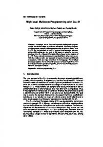
Simple Demo
• • • •
add #pragma omp parallel for -fopenmp export OMP_NUM_THREADS=10 omp_get_wtime()
speed up 40
30
speed-up
20
10
0
0
12.5
25.0
37.5
50.0
threads 4
Simple Demo
•
“#pragma omp parallel for” works for ‣ ‣ ‣ ‣
signed integer loops simple comparisons with loop invariant integers 3.expression invariant increment/decrement single entry / single exit loop
5
Private vs Shared Variables
•
default: ‣ ‣
•
all variables are shared among processes expect: index variable in “parallel for” (if declared there)
otherwise has to be specified manually e.g.: ‣
#pragma omp parallel for private (x, y, z)
6
Some Special Commands
7
Some Environment Variables
8
Local Interest Points
9
Applications of Local Invariant Features
• • • • • •
Wide baseline stereo Motion tracking Panoramas Mobile robot navigation 3D reconstruction Recognition ‣ ‣ ‣
•
Specific objects Textures Categories
…
Slide credit: Kristen Grauman
Wide-Baseline Stereo
Image from T. Tuytelaars ECCV 2006 tutorial
Recognition of Categories Constellation model
Bags of words
Csurka et al. (2004) Dorko & Schmid (2005) Sivic et al. (2005) Lazebnik et al. (2006), …
Weber et al. (2000) Fergus et al. (2003)
Slide credit: Svetlana Lazebnik
B. Leibe
45
Application of Point Correspondence: Image Matching
by Diva Sian
by swashford Slide credit: Steve Seitz 13
Harder Case
by Diva Sian
by scgbt
Slide credit: Steve Seitz 14
Harder Still?
NASA Mars Rover images Slide credit: Steve Seitz 15
Answer Below (Look for tiny colored squares)
Slide credit: Steve Seitz
NASA Mars Rover images with SIFT feature matches (Figure by Noah Snavely) 16
Application: Image Stitching
Slide credit: Darya Frolova, Denis Simakov 17
Application: Image Stitching
•
Procedure: ‣
Detect feature points in both images
Slide credit: Darya Frolova, Denis Simakov 18
Application: Image Stitching
•
Procedure: ‣ ‣
Detect feature points in both images Find corresponding pairs Slide credit: Darya Frolova, Denis Simakov 19
Application: Image Stitching
•
Procedure: ‣ ‣ ‣
Detect feature points in both images Find corresponding pairs Use these pairs to align the images Slide credit: Darya Frolova, Denis Simakov 20
Application: Image Stitching
•
Procedure: ‣ ‣ ‣
Detect feature points in both images Find corresponding pairs Use these pairs to align the images Slide credit: Darya Frolova, Denis Simakov 21
Automatic Mosaicing
[Brown & Lowe, ICCV’03]
22
Panorama Stitching
[Brown, Szeliski, and Winder, 2005]
http://www.cs.ubc.ca/~mbrown/autostitch/autostitch.html
iPhone version available
23
Point Correspondence for Object Instance Recognition: General Approach 1. Find a set of distinctive keypoints
B3
A1 A2
A3
B2 B1
N pixels
Similarity measure
e.g. color
e.g. color
2. Extract and normalize the region content 3. Compute a local descriptor from the normalized region 4. Match local descriptors
N pixels
24
Recognition of Specific Objects, Scenes
Schmid and Mohr 1997
Rothganger et al. 2003
Sivic and Zisserman, 2003
Lowe 2002 25
1. Interest Point Detection Common Requirements
•
Problem 1: ‣
Detect the same point independently in both images
No chance to match!
We need a repeatable detector! Slide credit: Darya Frolova, Denis Simakov 26
1. Interest Point Detection Common Requirements
•
Problem 1: ‣
•
Detect the same point independently in both images
Problem 2: ‣
For each point correctly recognize the corresponding one
?
We need a reliable and distinctive descriptor! Slide credit: Darya Frolova, Denis Simakov 27
1. Interest Point Detection Requirements • Region extraction needs to be repeatable and accurate Ø
Invariant to translation, rotation, scale changes
Ø
Robust or covariant to out-of-plane (≈affine) transformations
Ø
Robust to lighting variations, noise, blur, quantization
• Locality: Features are local, therefore robust to occlusion and clutter. • Quantity: We need a sufficient number of regions to cover the object. • Distinctiveness: The regions should contain “interesting” structure. • Efficiency: Close to real-time performance.
28
1. Interest Point Detection Many Existing Detectors Available • • • • • • • •
Hessian & Harris Laplacian, DoG Harris-/Hessian-Laplace Harris-/Hessian-Affine EBR and IBR
[Beaudet ‘78], [Harris ‘88] [Lindeberg ‘98], [Lowe ‘99] [Mikolajczyk & Schmid ‘01] [Mikolajczyk & Schmid ‘04] [Tuytelaars & Van Gool ‘04]
MSER
[Matas ‘02]
Salient Regions
[Kadir & Brady ‘01]
Others…
• Those detectors have become a basic building block for many recent applications in Computer Vision.
29
1. Interest Point Detection Automatic Scale Selection • Normalize: Rescale to fixed size
30
1. Interest Point Detection Characteristic Scale • We define the characteristic scale as the scale that produces peak of Laplacian response
Characteristic scale T. Lindeberg (1998). "Feature detection with automatic scale selection." International Journal of Computer Vision 30 (2): pp 77--116. Slide credit: Svetlana Lazebnik 31
Laplacian-of-Gaussian (LoG) • Interest points: Ø
Local maxima in scale space of Laplacian-ofGaussian
σ5
σ4
σ3 σ2
σ Slide adapted from Krystian Mikolajczyk 32
Laplacian-of-Gaussian (LoG) • Interest points: Ø
Local maxima in scale space of Laplacian-ofGaussian
σ5
σ4
σ3 σ2
σ Slide adapted from Krystian Mikolajczyk 33
Laplacian-of-Gaussian (LoG) • Interest points: Ø
Local maxima in scale space of Laplacian-ofGaussian
σ5
σ4
σ3 σ2
σ Slide adapted from Krystian Mikolajczyk 34
Laplacian-of-Gaussian (LoG) • Interest points: Ø
Local maxima in scale space of Laplacian-ofGaussian
σ5
σ4
σ3 σ2
σ
⇒ List of (x, y, σ)
Slide adapted from Krystian Mikolajczyk 35
LoG Detector: Workflow
Slide credit: Svetlana Lazebnik 36
LoG Detector: Workflow
Slide credit: Svetlana Lazebnik 37
LoG Detector: Workflow
Slide credit: Svetlana Lazebnik 38
Technical Detail
•
We can efficiently approximate the Laplacian with a difference of Gaussians:
(Laplacian)
(Difference of Gaussians)
39
Difference-of-Gaussian (DoG)
•
Difference of Gaussians as approximation of the LoG ‣
•
This is used e.g. in Lowe’s SIFT pipeline for feature detection.
Advantages ‣ ‣
No need to compute 2nd derivatives Gaussians are computed anyway, e.g. in a Gaussian pyramid.
-
=
40
DoG – Efficient Computation • Computation in Gaussian scale pyramid
Sampling with step σ4 =2 σ σ σ Original image
σ
Slide adapted from Krystian Mikolajczyk 41
Key point localization with DoG (Lowe)
•
Detect maxima of difference-ofGaussian (DoG) in scale space
•
Then reject points with low contrast (threshold)
•
Eliminate edge responses
Candidate keypoints: list of (x,y,σ) Slide credit: David Lowe 42
Results: Lowe’s DoG
43
Example of Keypoint Detection (a) 233x189 image (b) 832 DoG extrema (c) 729 left after peak value threshold (d) 536 left after testing ratio of principle curvatures (removing edge responses)
Slide credit: David Lowe 44
Summary: Scale Invariant Detection • Given: Two images of the same scene with a large scale difference between them.
• Goal: Find the same interest points independently in each image. • Solution: Search for maxima of suitable functions in scale and in space (over the image).
• Two strategies Ø Ø
Ø
Laplacian-of-Gaussian (LoG) Difference-of-Gaussian (DoG) as a fast approximation These can be used either on their own, or in combinations with singlescale keypoint detectors (Harris, Hessian).
45
DoG Code
46
Scheduling (parallelizing octaves)
•
Load balancing problem
•
Scheduling
47
Cost of scheduling
48
Overhead of threading #pragma omp parallel for for ( k = 0; k < m; k++ ) { fn1(k); fn2(k); } #pragma omp parallel for // adds unnecessary overhead for ( k = 0; k < m; k++ ) { fn3(k); fn4(k); }
1 x overhead
vs. #pragma omp parallel { #pragma omp for for ( k = 0; k < m; k++ ) { fn1(k); fn2(k); } #pragma omp for for ( k = 0; k < m; k++ ) { fn3(k); fn4(k); } }
2 x overhead
49
More modifiers •
#pragma omp parallel for no wait ‣
•
doesn’t wait for jobs to finish
#pragma omp master ‣
•
only master thread executes
#pragma omp barrier ‣
•
explicit synchonization
#pragma omp single ‣
•
only one thread executes
#pragma omp critical ‣
only one thread can enter (risk of deadlocks)
‣
named critical sections #pragma omp critical (name)
•
#pragma omp atomic ‣
•
thread cannot be interrupted #pragma omp parallel if (n>=16)
‣
parallel only for more than 16 loops 50
Additional resources:
•
http://www.drdobbs.com/parallel/openmp-a-portable-solution-forthreading/225702895?pgno=1
•
http://www.compunity.org/training/tutorials/ 2%20Basic_Concepts_Parallelization.pdf
•
http://www.vlfeat.org/api/sift.html
•
http://www.cs.ubc.ca/~lowe/papers/ijcv04.pdf
51