Introduction to Numerical Algebraic Geometry∗ Andrew J. Sommese†
Jan Verschelde‡
Charles W. Wampler§
14 April 2003 Abstract. In a 1996 paper, Andrew Sommese and Charles Wampler began developing a new area, “Numerical Algebraic Geometry”, which would bear the same relation to “Algebraic Geometry” that “Numerical Linear Algebra” bears to “Linear Algebra”. To approximate all isolated solutions of polynomial systems, numerical path following techniques have been proven reliable and efficient during the past two decades. In the nineties, homotopy methods were developed to exploit special structures of the polynomial system, in particular its sparsity. For sparse systems, the roots are counted by the mixed volume of the Newton polytopes and computed by means of polyhedral homotopies. In Numerical Algebraic Geometry we apply and integrate homotopy continuation methods to describe solution components of polynomial systems. One special, but important problem in Symbolic Computation concerns the approximate factorization of multivariate polynomials with approximate complex coefficients. Our algorithms to decompose positive dimensional solution sets of polynomial systems into irreducible components can be considered as symbolic-numeric, or perhaps rather as numeric-symbolic, since numerical interpolation methods are applied to produce symbolic results in the form of equations describing the irreducible components. Applications from mechanical engineering motivated the development of Numerical Algebraic Geometry. The performance of our software on several test problems illustrate the effectiveness of the new methods.
1
Introduction
The goal of this paper is to provide an overview of the main ideas developed so far in our research program to implement numerical algebraic geometry, initiated in [86]. We are concerned with numerically solving polynomial systems. While the homotopy continuation methods of the past were limited to approximating only the isolated roots, we developed tools to describe all positive dimensional irreducible components of the solution set of a polynomial system. In particular, our algorithms produce for every irreducible component a witness ∗ An
outline of notes for the CIMPA Graduate School, near Buenos Aires, Argentina, 14-25 July 2003. of Mathematics, University of Notre Dame, Notre Dame, IN 46556-4618, USA. Email:
[email protected] URL: http://www.nd.edu/˜sommese. This material is based upon work supported by the National Science Foundation under Grant No. 0105653; and the Duncan Chair of the University of Notre Dame. ‡ Department of Mathematics, Statistics, and Computer Science, University of Illinois at Chicago, 851 South Morgan (M/C 249), Chicago, IL 60607-7045, USA. Email:
[email protected] or
[email protected] URL: http://www.math.uic.edu/˜jan. This material is based upon work supported by the National Science Foundation under Grant No. 0105739 and Grant No. 0134611. § General Motors Research and Development, Mail Code 480-106-359, 30500 Mound Road, Warren, MI 480909055, USA. Email:
[email protected]. † Department
set, whose cardinality equals the degree of the component, as this set is obtained by intersecting the component with a general linear space of complementary dimension. A point of a witness set corresponds to what is known in algebraic geometry as a generic point. Our main results [77, 78, 79, 80, 81, 82, 83, 84, 85] can be summarized in four items: 1. In [77] we presented a cascade of homotopies to find candidate witness points for every component of the solution set. Separating the junk from the candidate witness points was done in [78], where factorization methods based on interpolation implemented a numerical irreducible decomposition. The use of central projections and a homotopy membership test to filter junk were the improvements of [79]. 2. An open problem in symbolic-numerical computing is the factorization of multivariate polynomials with approximate coefficients [38]. While we first struggled with the same challenge, the discovery of monodromy [80] followed by the validation by the linear trace [81] enabled us to deal with very high degree components, using only machine floating point numbers. In [82] we defined these methods for multiple components and applied it to the factorization of multivariate polynomials in [85]. 3. Our new homotopy algorithms have been implemented and tested using the path trackers in the software package PHCpack [93]. In [84] we outlined the new tools in PHCpack and describe a simple interface to Maple. Our software found the degrees of all irreducible components of the cyclic 8 and 9 roots problems, which previously could only be done via Gr¨ obner bases (and only by the very best implementation [18]). 4. Polynomial systems with positive dimensional components occur naturally when designing mechanical devices which permit motion. We investigated a special case of a moving platform, discovering through a numerical irreducible decomposition [81] a component missed by experts [36]. This and other applications of our tools to systems coming from mechanical design are described in [83]. In this paper we will introduce these results, after first describing homotopy continuation methods in the next section. Recent and exciting new developments in fields related to numerical algebraic geometry will not be explained, but we cannot refrain from mentioning numerical Schubert calculus ([32], [34], [55], [91], [102]) and numerical jet geometry [70]. Acknowledgements. The authors thank Alicia Dickenstein and Ioannis Emiris for their invitation to present their work at the summer school.
2
Homotopy Continuation Methods
Homotopy continuation methods operate in two stages. Firstly, homotopy methods exploit the structure of the system f (x) = 0 to find a root count and to construct a start system g(x) = 0 that has exactly as many regular solutions as the root count. This start system is embedded in the homotopy h(x, t) = γ(1 − t)g(x) + tf (x) = 0, t ∈ [0, 1], (1) with γ ∈ C a random number. Secondly, as t moves from 0 to 1, numerical continuation methods trace the paths that originate at the solutions of the start system towards the solutions of the target system. The good properties we expect from a homotopy are (borrowed from [45]):
1. (triviality) The solutions for t = 0 are trivial to find. 2. (smoothness) No singularities along the solution paths occur (because of γ). 3. (accessibility) An isolated solution of multiplicity m is reached by exactly m paths. Continuation or path-following methods are standard numerical techniques ([1, 2, 3], [57], [107, 108]) to trace the solution paths defined by the homotopy using predictor-corrector methods. The smoothness property of complex polynomial homotopies implies that paths never turn back, so that during correction the parameter t stays fixed, which simplifies the set up of path trackers. The adaptive step size control determines the step length while enforcing quadratic convergence in Newton’s method to avoid path crossing. At the end of the path, end games ([33], [62, 63, 64], [87]) deal with diverging paths and paths leading to singular roots. Following [32], we say that a homotopy is optimal if every path leads to one solution. The classification in Table 1 (from [94]) contains key words for three classes of polynomial systems for which optimal homotopies are available in PHCpack [93]. These homotopies have no diverging paths for generic instances of polynomial systems in their class. system dense sparse determinantal
model highest degrees Newton polytopes localization posets
theory B´ezout Bernshteˇın Schubert
Pn (C∗ )n Gmr
space projective toric Grassmannian
Table 1: Key words of the three classes of polynomial systems. The earliest applications of homotopies for solving polynomial systems ([8], [15], [24], [25], [43], [47] [56], [113], [114]) belong to the dense class, where the number of paths equals the product of the degrees in the system. Multi-homogeneous homotopies were introduced in [58, 59] and applied in [103, 104], see also [105]. Similar are the random product homotopies [48, 49], see also [44] and [51]. Methods to construct linear-product start systems were introduced in [96], and extended in [97, 98], [54] and [112]. A general approach to exploit product structures was developed in [65]. Almost all systems have fewer terms than allowed by their degrees. Implementing constructive proofs of Bernshteˇın’s theorems [5], polyhedral homotopies were introduced in [30] and [101] to solve sparse systems more efficiently. These methods provided ways to start cheater’s homotopies ([50], [52]) and special instances of coeffient-parameter polynomial continuation ([60, 61]). The root count requires the calculation of the mixed volume, for which a lift-and-prune approach was presented in [16]. Exploitation of symmetry was studied in [99] and the dynamic lifting of [100] led to incremental polyhedral continuation. See [95] for a Toric Newton. Extensions to count all affine roots (also those with zero components) were proposed in in [17], [23], [31], [53], [71, 72], [73]. Very efficient calculations of mixed volumes are described in [13], [21, 22], [40], [46], and [92]. Determinantal systems (with equations like det(A|X) = 0) arise in problems of enumerative geometry. The homotopies in numerical Schubert calculus first appeared explicitly in [32], originating from questions in real enumerative geometry [88, 89]. While real enumerative geometry [90] is interesting on its own, these homotopies solve the pole placement problem ([6], [68, 69], [74], [75]) in control theory. Recent improvements and applications can be found in [34], [55], [91], and [102]. We end this section noting that homotopies have a wider application range than “just” solving polynomial systems, see for instance [109] for a survey, [110], and [111] for a description of HOMPACK. The speedup of continuation methods on multi-processor machines has been addressed in [4, 7, 29].
3
A Dictionary
Kempf writes in [39] that “Algebraic geometry studies the delicate balance between the geometrically plausible and the algebraically possible”. With our numerical tools, we feel closer to the geometrical than to the algebraic side, because we are not calculating with polynomials in the algebraic sense. In [84] we outlined the structure of a dictionary, presented as Table 2.
Algebraic Geometry variety
irreducible variety generic point on an irreducible variety pure dimensional variety irreducible decomposition of a variety
Numerical Algebraic Geometry Dictionary example Numerical in 3-space Analysis collection of points, polynomial system algebraic curves, and + union of witness sets, see below algebraic surfaces for the definition of a witness point a single point, or polynomial system a single curve, or + witness set a single surface + probability-one membership test random point on point in a witness set; a witness point an algebraic is a solution of polynomial system on the curve or surface variety and on a random slice whose codimension is the dimension of the variety one or more points, or polynomial system one or more curves, or + set of witness sets of same dimension one or more surfaces + probability-one membership tests several pieces polynomial system of different + array of sets of witness sets and dimensions probability-one membership tests
Table 2: Dictionary to translate algebraic geometry into numerical analysis. The probability-one membership test determines whether a given point p lies on a pure dimensional solution set. Suppose we have witness points defined by a polynomial system f (x) = 0 and hyperplanes L(x) = 0. A homotopy method implements the probability-one membership test: 1. Define K(x) = L(x) − L(p). As K(p) = 0, the hyperplanes K pass through p. 2. Consider the homotopy h(x, t) =
µ
f (x) K(x)
¶
(1 − t) +
µ
f (x) L(x)
¶
t = 0.
(2)
At t = 1 we start tracking paths at the witness set and find their end points at t = 0. 3. If p belongs to the solution set of h(x, 0) = 0, then it is also a witness point of the pure dimensional solution set. Notice that this test does not move the point p, which may be a highly singular point. This observation is important for the numerical stability of this test.
4
Witness Sets and a Cascade of Homotopies
A witness set is the basic concept of numerical algebraic geometry as it allows us to apply numerical methods for isolated solutions to positive dimensional solution components. Every irreducible component of a solution set is presented by a witness set whose cardinality equals the degree of the irreducible component. To reduce a solution set of dimension k to a set of isolated points, we cut the k degrees of freedom by adding k random hyperplanes L(x) = 0 to the system f (x) = 0 which defines the entire solution set. One obstacle is that we have to deal with systems whose number of equations in not necessarily the same as the number of unknowns. If there are fewer equations than unknowns, we simply add enough random hyperplanes to make up for the difference, so underdetermined systems are easy to handle. Let us consider overdetermined systems, say f consists of 5 equations in 3 variables. To turn f into a system of N equations in N variables where N is either 3 or 5, we can respectively apply the following techniques: randomization: Choosing random complex numbers aij , we add random combinations of the last two polynomial to the first three polynomials: f1 (x) + a11 f4 (x) + a12 f5 (x) = 0 f2 (x) + a21 f4 (x) + a22 f5 (x) = 0 (3) f3 (x) + a31 f4 (x) + a32 f5 (x) = 0 slack variables: We introduce two new variables z1 and z2 (so-called slack variables) and add random multiples of these variables to every equation: f1 (x) + a11 z1 + a12 z2 = 0 f2 (x) + a21 z1 + a22 z2 = 0 f3 (x) + a31 z1 + a32 z2 = 0 (4) f (x) + a z + a z = 0 4 41 1 42 2 f5 (x) + a51 z1 + a52 z2 = 0
While the randomization technique might seem at first more attractive because we are left with fewer equations, working with slack variables provides a cascade of homotopies to compute candidate witness points on all positive dimensional components. In particular, considering f4 and f5 as hyperplanes L1 and L2 to cut the solution set of the first three equation in f , we have the following systems in the cascade: f1 (x) + a11 z1 + a12 z2 = 0 f1 (x) + a11 z1 + a12 z2 = 0 f1 (x) + a11 z1 = 0 f2 (x) + a21 z1 = 0 f2 (x) + a21 z1 + a22 z2 = 0 f2 (x) + a21 z1 + a22 z2 = 0 f3 (x) + a31 z1 + a32 z2 = 0 f3 (x) + a31 z1 + a32 z2 = 0 f3 (x) + a31 z1 = 0 (5) z1 = 0 L1 (x) + z1 = 0 L1 (x) + z1 = 0 z2 = 0 z2 = 0 L2 (x) + z2 = 0
We start with the largest system at the left. Solutions with z1 = 0 and z2 = 0 define witness points on the two dimensional solution components. Solutions with z1 6= 0 and z2 6= 0 provide start points in the homotopy which removes L2 from the system. The paths defined by this move end at witness points on the one dimensional components, picked out by z1 = 0. Solutions with z1 6= 0 are used in the homotopy which removes L1 to lead to the isolated solutions of the systems. We next give a specific example of this cascade.
5
A Numerical Irreducible Decomposition
Consider the following example:
(x1 − 1)(x2 − x21 ) = 0 (x1 − 1)(x3 − x31 ) = 0 f (x) = 2 (x1 − 1)(x2 − x21 ) = 0
(6)
From its factored form we see that f (x) = 0 has two solution components: the two dimensional plane x1 = 1 and the twisted cubic { (x1 , x2 , x3 ) | x2 − x21 = 0, x3 − x31 = 0 }. To describe the solution set of this system, we use a cascade of homotopies, the chart in Figure 1 illustrates the flow of data for this example. Because the top dimensional component is of dimension two, we add two random hyperplanes to the system and make it square again by adding two slack variables z1 and z2 : (x1 − 1)(x2 − x21 ) + a11 z1 + a12 z2 = 0 (x1 − 1)(x3 − x31 ) + a21 z1 + a22 z2 = 0 (x21 − 1)(x2 − x21 ) + a31 z1 + a32 z2 = 0 (7) e(x, z1 , z2 ) = c + c x + c x + c x + z = 0 10 11 1 12 2 13 3 1 c20 + c21 x1 + c22 x2 + c23 x3 + z2 = 0
where all constants aij , i = 1, 2, 3, j = 1, 2, and ckl , k = 1, 2, l = 0, 1, 2, 3 are randomly chosen complex numbers. Observe that when z1 = 0 and z2 = 0 the solutions to e(x, z1 , z2 ) = 0 satisfy f (x) = 0. So if we solve e(x, z1 , z2 ) = 0 we will find a single witness point on the two dimensional solution component x1 = 1 as a solution with z1 = 0 and z2 = 0. Using polyhedral homotopies, this requires the tracing of six solutions paths. The embedding was proposed in [77] to find generic points on all positive dimensional solution components with a cascade of homotopies. In [77] it was proven that solutions with slack variables zi 6= 0 are regular and, moreover, that those solutions can be used as start solutions in a homotopy to find witness points on lower dimensional solution components. At each stage of the algorithm, we call solutions with nonzero slack variables nonsolutions. In the solution of e(x, z1 , z2 ) = 0, one path ended with z1 = 0 = z2 , the five other paths ended in regular solutions with z1 6= 0 and z2 6= 0. These five “nonsolutions” are start solutions for the next stage, which uses the homotopy h2 (x, z1 , z2 , t) =
(x1 − 1)(x2 − x21 ) + a11 z1 + a12 z2 = 0 (x1 − 1)(x3 − x31 ) + a21 z1 + a22 z2 = 0 (x21 − 1)(x2 − x21 ) + a31 z1 + a32 z2 = 0 c10 + c11 x1 + c12 x2 + c13 x3 + z1 = 0 z2 (1 − t) + (c20 + c21 x1 + c22 x2 + c23 x3 + z2 )t = 0
(8)
where t goes from one to zero, replacing the last hyperplane with z2 = 0. Of the five paths, four of them converge to solutions with z1 = 0. Of those four solutions, one of them is found to lie on the two dimensional solution component x1 = 1, the other three are generic points on the twisted cubic. As there is one solution with z1 6= 0, we have one candidate left to use as a start point in the final stage, which searches for isolated solutions of f (x) = 0. The homotopy for this stage is (x1 − 1)(x2 − x21 ) + a11 z1 = 0 (x1 − 1)(x3 − x31 ) + a21 z1 = 0 h1 (x, z1 , t) = (9) (x21 − 1)(x2 − x21 ) + a31 z1 = 0 z1 (1 − t) + (c10 + c11 x1 + c12 x2 + c13 x3 + z1 )t = 0
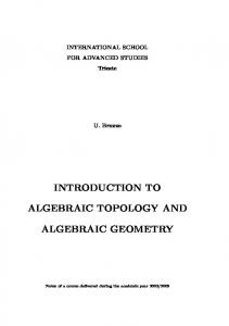
which as t goes from 1 to 0, replaces the last hyperplane z1 = 0. At t = 0, the solution is found to lie on the twisted cubic, so there are no isolated solutions. The calculations are summarized in Figure 1. The breakup into irreducibles will be explained in the next section. WitnessGenerate Path following
l e v e l
WitnessClassify Filter Points
Breakup into
Irreducibles ¶ ³ ³ ¶ Homotopy + Start Solutions Filter = ∅ µ ´ µ ´ ? - 0 at infinity 6 paths ? c2 W - 1 to classify W2- 1 on x1 = 1 = W21 1 solutions 5 nonsolutions
Append to Filter
2 l e v e l
? 5 paths
-
0 at infinity 4 solutions 1 nonsolution
1 l e v e l
? 1 on x c 1 = 1 = J1 W13 to classify W1
3 on cubic
= W11
Append to Filter
? 1 path
-
0 at infinity 1 solution
0
? 0 on x c 1 =1 W01 on cubic
= J0
Figure 1: Numerical Irreducible Decomposition of a system whose solutions are the 2-dimensional plane x1 = 1, the twisted cubic, and one isolated point. At level i, for i = 2, 1, 0, we filter candidate ci into junk sets Ji and witness sets Wi . The sets Wi are partitioned into witness witness sets W sets Wij for the irreducible components.
6
Factorization Methods
A recent trend in computer algebra is the adaption of symbolic methods to deal with approximate input data, which leads to the use of hybrid methods [12]. One such problem is the factor of multivariate polynomials, listed as a challenge in [38]. Recent papers on this problem are [9, 10], [19, 20], [37], and [76].
6.1
Monodromy to Partition Witness Point Sets
We can see whether a curve factors or not by looking at its plot in complex space, i.e.: we consider the curve as a Riemann surface. Figure 2 was made with Maple (see [11] for instructions).
1 2 0.5 Re(z^1/3)
1
0 0
–0.5
Im(z)
–1
–1 –2
–1
0 Re(z)
1
2
–2
Figure 2: The Riemann surface of z 3 −w = 0. The height of the surface is the real part of w = z 1/3 , while the gray scale corresponds to the imaginary part of w = z 1/3 . Observe that a loop around the origin permutes the order of points. Looking at Figure 2, imagine a line which intersects the surface in three points. Taking one complete turn of the line around the vertical axis z = 0 will cause the points to permute. For example, the point which was lowest will have moved up, while another point will have come down. Such a permutation can only happen if the corresponding algebraic curve is irreducible. Based on this observation, we can decompose any pure dimensional set into irreducible components. Our monodromy algorithm returns a partition of the witness set for a pure dimensional component: points in the same subset of the partition belong to the same irreducible component. Recall that witness points are defined by a system f (x) = 0 and a set of hyperplanes L(x) = 0. With the homotopy ¶ ¶ µ µ f (x) f (x) t = 0, λ ∈ C, (10) (1 − t) + hKL (x, t) = λ L(x) K(x) we find new witness points on the hyperplanes K(x) = 0, starting at those witness points satisfying L(x) = 0, letting t move from one to zero. Choosing another random constant µ 6= λ, we move back from K to L, using the homotopy µ ¶ µ ¶ f f hLK (x, t) = µ (1 − t) + t = 0, µ ∈ C. (11) L K
The homotopies hKL (x, t) = 0 and hLK (x, t) = 0 implement one loop in the monodromy algorithm, moving witness points from L to K and then back from K to L. At the end of the loop we have the same witness set as the set we started with, except possibly permuted. Permuted points belong the same irreducible component. Notice that the monodromy algorithm does not know the locations of the singularities. See [14] for the algorithms to compute the monodromy group of an algebraic curve in Maple (package algcurves).
6.2
Linear Traces to Validate the Partition
When we run the monodromy algorithm, we may not have made enough loops to group as many witness points as the degree of each factor, i.e.: the partition predicted by the monodromy might be too fine. For a k-dimensional solution component, it suffices to consider a curve on the component cut out by k − 1 random hyperplanes. The factorization of the curve tells the decomposition of the solution component. Therefore, we restrict our explanation of using the linear trace to the case of a curve in the plane. Suppose we have three points in the plane obtained as (projections of) witness points from some polynomial system. If the monodromy found loops between those points, then we know that these points lie on an irreducible factor of degree at least three. Whence our question: is this irreducible factor on which the given three points lie of degree three? To answer this question we represent the factor by a cubic polynomial f in the form f (x, y(x))
= (y − y1 (x))(y − y2 (x))(y − y3 (x)) = y 3 − t1 (x)y 2 + t2 (x)y − t3 (x)
(12)
Since deg(f ) = 3, deg(t1 ) = 1, so t1 is the linear trace: t1 (x) = c1 x + c0 . We now proceed as follows. Via interpolation we find the coefficients c0 and c1 . We first sample the cubic at x = x0 and x = x1 . The samples are {(x0 , y00 ), (x0 , y01 ), (x0 , y02 )} and {(x1 , y10 ), (x1 , y11 ), (x1 , y12 )}. To find c0 and c1 we then solve the linear system ½ y00 + y01 + y02 = c1 x0 + c0 (13) y10 + y11 + y12 = c1 x1 + c0 With t1 we can predict the sum of the y’s for a fixed choice of x. For example, samples at x = x2 are {(x2 , y20 ), (x2 , y21 ), (x2 , y22 )}. So our test consists in computing t1 (x2 ) in two ways: c1 x2 + c0 = y20 + y21 + y22 .
(14)
If the equality holds, then the answer to our question is yes.
6.3
Efficiency and Numerical Stability
The validation with the linear trace is fast. Therefore, our implementation does this validation each time a new loop with the monodromy algorithm is found. Even as we do not know the locations of the singularities, practical experiences on many systems all lead to a rapid finding of permutations. While this approach is suitable for irreducible factors of very large degree (e.g., one thousand), strategies purely based on traces perform often better for smaller degrees. Related to the efficiency is the good numerical stability: if we can compute witness points with standard machine arithmetic, then we can also factor using standard machine arithmetic. This feature is very important when the accuracy of coefficients of the polynomial system is limited.
7
Software
We agree with the statement: “It can be argued that the “mission” of numerical analysis is to provide the scientific community with effective software tools.” (taken from the preface to [26]). Aside from our missionary intentions, software has helped us refining our algorithms, along the lines of the quote (from [41]): “Another reason that programming is harder than the writing of books and research papers is that programming demands a significant higher standard of accuracy.” The software package PHCpack [93] is currently undergoing the transition from being a toolbox/blackbox for various homotopy continuation methods to approximate all isolated solutions to a complete solving environment with capabilities to handle positive dimensional solution components efficiently, both in terms of computer operations and user manipulations. By the latter we hint at the search to find the right user interface, identifying the right data flow and trying to balance the toolbox with the blackbox approach. While PHCpack offered the first reliable implementation of polyhedral homotopies, its efficiency is currently surpassed by the implementations described in [21, 22, 46] and [13, 28, 40, 92]. To interact better with other codes, we are currently developing an interface from the Ada routines in PHCpack to routines written in C. Another (but related) interface concerns the interaction with computer algebra software. In [84] we describe a very simple interface to Maple.
8
Applications
A benchmark suite for systems with positive dimensional solution components is gradually taking shape. Rather than listing summaries of a benchmark, we choose to treat two very typical applications: the cyclic n-roots problem from computer algebra and a special Stewart-Gough platform from mechanical design. The cyclic n-roots problem. This problem is already interesting by its compact formulation and widespread fame in the computer algebra community, but by known theoretical results concerning the number of isolated roots when n is prime. For n = 8, there are 16 one dimensional irreducible components: eight quadrics and eight curves of degree 16. While approximations to all 1,152 isolated cyclic 8-roots were found already in the first release of PHCpack, monodromy was needed to factor the curve of degree 144 into irreducibles. To compute all witness points for the cyclic 9-roots problem, the software of [46] was essential. While the factorization of a two dimensional component of degree 18 into six cubics posed no difficulty, the homotopy membership test was required to certify that among the 6,642 isolated ones 162 cyclic 9-roots occured with multiplicity four. In addition, multi-precision arithmetic was used to confirm this result. The isolated cyclic n-roots (up to n = 13, for which 2,704,156 paths were traced) can be found on http://www.is.titech.ac.jp/~kojima/polynomials/cyclic13. These roots have been computed with PHoM [28]. A special Stewart-Gough platform. The Stewart-Gough platform is a parallel robot which attracted lots of interest from computational kinematicians and researchers in computer algebra. That the platform has forty isolated solutions was first established computationally by continuation [67] and elimination methods [42, 66], later proved analytically in [35] and [106]. A six-legged platform (similar to the general Stewart-Gough platform) which permits motion was presented by [27] and first analyzed in [36]. Instead of forty isolated solutions we now
consider a curve. In our formulation of the two cases we studied, twelve lines corresponded to degenerate cases deemed uninteresting from a mechanisms point of view. In the first case we were then left with one irreducible component of degree 28, while in the second case we found five components, four of degree six (one sextic was missed by the analysis of [36]), and one component of degree four, see Figure 3.
Figure 3: One component of the Griffis-Duffy platform. Starting at the configuration at the left above, we see the clockwise rotation of the end platform. It is interesting to note that the running times for the factorization with the monodromytraces method does not seem to depend on the particular geometry of the system, i.e.: the execution times are about the same in both cases, when we deal with one irreducible factor of high degree or with several factors of smaller degrees.
References [1] E.L. Allgower and K. Georg. Numerical Continuation Methods, an Introduction, volume 13 of Springer Ser. in Comput. Math. Springer–Verlag, 1990. To appear in the SIAM Classics in Applied Mathematics Series. [2] E.L. Allgower and K. Georg. Continuation and path following. Acta Numerica, pages 1–64, 1993. [3] E.L. Allgower and K. Georg. Numerical Path Following. In Techniques of Scientific Computing (Part 2), edited by P.G. Ciarlet and J.L. Lions volume 5 of Handbook of Numerical Analysis, pages 3–203. North-Holland, 1997. [4] D.C.S. Allison, A. Chakraborty, and L.T. Watson. Granularity issues for solving polynomial systems via globally convergent algorithms on a hypercube. J. of Supercomputing, 3:5–20, 1989. [5] D.N. Bernshteˇın. The number of roots of a system of equations. Functional Anal. Appl., 9(3):183–185, 1975. Translated from Funktsional. Anal. i Prilozhen., 9(3):1–4,1975.
[6] C.I. Byrnes. Pole assignment by output feedback. In Three Decades of Mathematical Systems Theory, edited by H. Nijmacher and J.M. Schumacher. Volume 135 of Lecture Notes in Control and Inform. Sci., pages 13–78. Springer–Verlag, 1989. [7] A. Chakraborty, D.C.S Allison, C.J. Ribbens, and L.T. Watson. The parallel complexity of embedding algorithms for the solution of systems of nonlinear equations. IEEE Transactions on Parallel and Distributed Systems 4(4): 458–465, 1993. [8] S.N. Chow, J. Mallet-Paret, and J.A. Yorke. Homotopy method for locating all zeros of a system of polynomials. In Functional differential equations and approximation of fixed points, edited by H.O. Peitgen and H.O. Walther. Volume 730 of Lecture Notes in Mathematics, pages 77–88, Springer–Verlag, 1979. [9] R.M. Corless, M.W. Giesbrecht, M. van Hoeij, I.S. Kotsireas and S.M. Watt. Towards factoring bivariate approximate polynomials. In Proceedings of the 2001 International Symposium on Symbolic and Algebraic Computation (ISSAC 2001), edited by B. Mourrain, pages 85–92, ACM 2001. [10] R.M. Corless, A. Galligo, I.S. Kotsireas, and S.M. Watt. A geometric-numeric algorithm for factoring multivariate polynomials. In Proceedings of the 2002 International Symposium on Symbolic and Algebraic Computation (ISSAC 2002), edited by T. Mora, ACM 2002. [11] R.M. Corless and D.J. Jeffrey. Graphing elementary Riemann surfaces. SIGSAM Bulletin 32(1):11–17, 1998. [12] R.M. Corless, E. Kaltofen, and S.M. Watt. Hybrid methods. In Computer Algebra Handbook, edited by J. Grabmeier, E. Kaltofen, and V. Weispfenning, pages 112-125, Springer-Verlag, 2002. [13] Y. Dai, S. Kim and M. Kojima. Computing all nonsingular solutions of cyclic-n polynomial using polyhedral homotopy continuation methods. J. Comput. Appl. Math. 152(1-2): 83–97, 2003. [14] B. Deconinck and M. van Hoeij. Computing Riemann matrices of algebraic curves. Physica D 152:28–46, 2001. [15] F.J. Drexler. Eine Methode zur Berechnung s¨ amtlicher L¨ osungen von Polynomgleichungssystemen. Numer. Math., 29(1):45–58, 1977. [16] I.Z. Emiris and J.F. Canny. Efficient incremental algorithms for the sparse resultant and the mixed volume. J. Symbolic Computation, 20(2):117–149, 1995. [17] I.Z. Emiris and J. Verschelde. How to count efficiently all affine roots of a polynomial system. Discrete Applied Mathematics, 93(1):21–32, 1999. [18] J.C. Faug`ere. A new efficient algorithm for computing Gr¨ obner bases (F 4 ). Journal of Pure and Applied Algebra 139(1-3):61–88, 1999. Proceedings of MEGA’98, 22–27 June 1998, Saint-Malo, France.
[19] A. Galligo and D. Rupprecht. Semi-numerical determination of irreducible branches of a reduced space curve. In Proceedings of the 2001 International Symposium on Symbolic and Algebraic Computation (ISSAC 2001), edited by B. Mourrain, pages 137–142, ACM 2001. [20] A. Galligo and D. Rupprecht. Irreducible decomposition of curves. J. Symbolic Computation 33(5):661–677, 2002. [21] T. Gao and T.Y. Li. Mixed volume computation via linear programming. Taiwan J. of Math. 4, 599–619, 2000. [22] T. Gao and T.Y. Li. Mixed volume computation for semi-mixed systems. Discrete Comput. Geom. 29(2):257-277, 2003. [23] T. Gao, T.Y. Li, and X. Wang. Finding isolated zeros of polynomial systems in C n with stable mixed volumes. J. of Symbolic Computation 28(1-2): 187-211, 1999. [24] C.B. Garcia and W.I. Zangwill. Finding all solutions to polynomial systems and other systems of equations. Math. Programming, 16(2):159–176, 1979. [25] C.B. Garcia and T.Y. Li. On the number of solutions to polynomial systems of equations. SIAM J. Numer. Anal., 17(4):540–546, 1980. [26] G.H. Golub and C.F. Van Loan. Matrix Computations. First Edition. The Johns Hopkins University Press, 1983. [27] M. Griffis and J. Duffy. Method and apparatus for controlling geometrically simple parallel mechanisms with distinctive connections. US Patent 5,179,525, 1993. [28] T. Gunji, S. Kim, M. Kojima, A. Takeda, K. Fujisawa, and T. Mizutani. PHoM – a polyhedral homotopy continuation method for polynomial systems. Available via http://www.is.titech.ac.jp/~kojima/sdp.html. [29] S. Harimoto and L.T. Watson. The granularity of homotopy algorithms for polynomial systems of equations. In Parallel processing for scientific computing, edited by G. Rodrigue, pages 115–120. SIAM, 1989. [30] B. Huber and B. Sturmfels. A polyhedral method for solving sparse polynomial systems. Math. Comp., 64(212):1541–1555, 1995. [31] B. Huber and B. Sturmfels. Bernstein’s theorem in affine space. Discrete Comput. Geom., 17(2):137–141, 1997. [32] B. Huber, F. Sottile, and B. Sturmfels. Numerical Schubert calculus. J. Symbolic Computation 26(6):767–788, 1998. [33] B. Huber and J. Verschelde. Polyhedral end games for polynomial continuation. Numerical Algorithms, 18(1):91–108, 1998. [34] B. Huber and J. Verschelde. Pieri homotopies for problems in enumerative geometry applied to pole placement in linear systems control. SIAM J. Control Optim. 38(4):1265– 1287, 2000.
[35] M.L. Husty. An algorithm for solving the direct kinematics of general Stewart-Gough platforms. Mechanism Machine Theory, 31(4):365–380, 1996. [36] M.L. Husty and A. Karger. Self-motions of Griffis-Duffy type parallel manipulators Proc. 2000 IEEE Int. Conf. Robotics and Automation, CDROM, San Francisco, CA, April 24– 28, 2000. [37] Y. Huang, W. Wu, H.J. Stetter, and L. Zhi. Pseudofactors of multivariate polynomials. In Proceedings of the 2000 International Symposium on Symbolic and Algebraic Computation (ISSAC 2000), edited by C. Traverso, pages 161-168, 2000. [38] E. Kaltofen. Challenges of symbolic computation: my favorite open problems. J. Symbolic Computation 29(6): 891–919, 2000. [39] G.R. Kempf. Algebraic Varieties. Volume 172 of London Mathematical Society Lecture Note Series. Cambridge University Press, 1993. [40] S. Kim and M. Kojima. Numerical stability of path tracing in polyhedral homotopy continuation methods. Research Report B-390, Tokyo Institute of Technology, March 2003. Available via http://www.is.titech.ac.jp/~kojima/sdp.html. [41] D.E. Knuth. Theory and Practice II. In Selected Papers on Computer Science, pages 129-139. Cambridge University Press, 1996. Originally published in Bulletin of EATCS 27:15-21, 1985. [42] D. Lazard. Stewart platform and Gr¨ obner basis. In Proc. ARK, pages 136–142, Ferrare, September 1992. [43] T.Y. Li. On Chow, Mallet-Paret and Yorke homotopy for solving systems of polynomials. Bulletin of the Institute of Mathematics. Acad. Sin., 11:433–437, 1983. [44] T.Y. Li. Solving polynomial systems. The Mathematical Intelligencer, 9(3):33–39, 1987. [45] T.Y. Li. Numerical solution of multivariate polynomial systems by homotopy continuation methods. Acta Numerica 6:399–436, 1997. [46] T.Y. Li and X. Li. Finding mixed cells in the mixed volume computation. Found. Comput. Math. 1(2): 161–181, 2001. Software available at http://www.math.msu.edu/~li. [47] T.Y. Li and T. Sauer. Regularity results for solving systems of polynomials by homotopy method. Numer. Math., 50(3):283–289, 1987. [48] T.Y. Li, T. Sauer, and J.A. Yorke. Numerical solution of a class of deficient polynomial systems. SIAM J. Numer. Anal., 24(2):435–451, 1987. [49] T.Y. Li, T. Sauer, and J.A. Yorke. The random product homotopy and deficient polynomial systems. Numer. Math., 51(5):481–500, 1987. [50] T.Y. Li, T. Sauer, and J.A. Yorke. The cheater’s homotopy: an efficient procedure for solving systems of polynomial equations. SIAM J. Numer. Anal., 26(5):1241–1251, 1989. [51] T.Y. Li and X. Wang. Solving deficient polynomial systems with homotopies which keep the subschemes at infinity invariant. Math. Comp., 56(194):693–710, 1991.
[52] T.Y. Li and X. Wang. Nonlinear homotopies for solving deficient polynomial systems with parameters. SIAM J. Numer. Anal., 29(4):1104–1118, 1992. [53] T.Y. Li and X. Wang. The BKK root count in C n . Math. Comp., 65(216):1477–1484, 1996. [54] T.Y. Li, T. Wang, and X. Wang. Random product homotopy with minimal BKK bound. In The Mathematics of Numerical Analysis, edited by J. Renegar, M. Shub, and S. Smale, volume 32 of Lectures in Applied Mathematics, pages 503–512, AMS, 1996. Proceedings of the AMS-SIAM Summer Seminar in Applied Mathematics, Park City, Utah, July 17-August 11, 1995, Park City, Utah. [55] T.Y. Li, X. Wang, and M. Wu. Numerical Schubert calculus by the Pieri homotopy algorithm. SIAM J. Numer. Anal. 20(2):578–600, 2002. [56] A.P. Morgan. A method for computing all solutions to systems of polynomial equations. ACM Trans. Math. Softw., 9(1):1–17, 1983. [57] A. Morgan. Solving polynomial systems using continuation for engineering and scientific problems. Prentice-Hall, Englewood Cliffs, N.J., 1987. [58] A. Morgan and A. Sommese. A homotopy for solving general polynomial systems that respects m-homogeneous structures. Appl. Math. Comput., 24(2):101–113, 1987. [59] A. Morgan and A. Sommese. Computing all solutions to polynomial systems using homotopy continuation. Appl. Math. Comput., 24(2):115–138, 1987. Errata: Appl. Math. Comput. 51 (1992), p. 209. [60] A.P. Morgan and A.J. Sommese. Coefficient-parameter polynomial continuation. Appl. Math. Comput., 29(2):123–160, 1989. Errata: Appl. Math. Comput. 51:207(1992). [61] A.P. Morgan and A.J. Sommese. Generically nonsingular polynomial continuation. In Computational Solution of Nonlinear Systems of Equations, edited by E.L. Allgower and K. Georg, pages 467–493, AMS, 1990. [62] A.P. Morgan, A.J. Sommese, and C.W. Wampler. Computing singular solutions to nonlinear analytic systems. Numer. Math., 58(7):669–684, 1991. [63] A.P. Morgan, A.J. Sommese, and C.W. Wampler. Computing singular solutions to polynomial systems. Adv. Appl. Math., 13(3):305–327, 1992. [64] A.P. Morgan, A.J. Sommese, and C.W. Wampler. A power series method for computing singular solutions to nonlinear analytic systems. Numer. Math., 63:391–409, 1992. [65] A.P. Morgan, A.J. Sommese, and C.W. Wampler. A product-decomposition theorem for bounding B´ezout numbers. SIAM J. Numer. Anal., 32(4):1308–1325, 1995. [66] B. Mourrain. The 40 generic positions of a parallel robot. In Proceedings of the 1993 International Symposium on Symbolic and Algebraic Computation (ISSAC 1993), edited by M. Bronstein, pages 173–182, ACM 1993. [67] M. Raghavan. The Stewart platform of general geometry has 40 configurations. ASME J. Mech. Design, 115:277–282, June 1993.
[68] M.S. Ravi, J. Rosenthal, and X. Wang. Dynamic pole placement assignment and Schubert calculus. SIAM J. Control and Optimization, 34(3):813–832, 1996. [69] M.S. Ravi, J. Rosenthal, and X. Wang. Degree of the generalized Pl¨ ucker embedding of a quot scheme and quantum cohomology. Math. Ann., 311:11–26, 1998. [70] G. Reid, C. Smith, and J. Verschelde. Geometric completion of differential systems using numeric-symbolic continuation. SIGSAM Bulletin 36(2):1–17, 2002. [71] J.M. Rojas. A convex geometric approach to counting the roots of a polynomial system. Theoret. Comput. Sci., 133(1):105–140, 1994. [72] J.M. Rojas. Toric intersection theory for affine root counting. Journal of Pure and Applied Algebra, 136(1):67–100, 1999. [73] J.M. Rojas and X. Wang. Counting affine roots of polynomial systems via pointed Newton polytopes. J. Complexity, 12:116–133, 1996. [74] J. Rosenthal. On dynamic feedback compensation and compactifications of systems. SIAM J. Control and Optimization, 32(1):279–296, 1994. [75] J. Rosenthal and J.C. Willems. Open problems in the area of pole placement. In Open Problems in Mathematical Systems and Control Theory, edited by V.D. Blondel, E.D. Sontag, M. Vidyasagar, and J.C. Willems, pages 181-191, Springer–Verlag, 1999. [76] T. Sasaki. Approximate multivariate polynomial factorization based on zero-sum relations. In Proceedings of the 2001 International Symposium on Symbolic and Algebraic Computation (ISSAC 2001), edited by B. Mourrain, pages 284–291, ACM 2001. [77] A.J. Sommese and J. Verschelde. Numerical homotopies to compute generic points on positive dimensional algebraic sets. Journal of Complexity 16(3):572–602, 2000. [78] A.J. Sommese, J. Verschelde and C.W. Wampler. Numerical decomposition of the solution sets of polynomial systems into irreducible components. SIAM J. Numer. Anal. 38(6):2022–2046, 2001. [79] A.J. Sommese, J. Verschelde, and C.W. Wampler. Numerical irreducible decomposition using projections from points on the components. In Symbolic Computation: Solving Equations in Algebra, Geometry, and Engineering, volume 286 of Contemporary Mathematics, edited by E.L. Green, S. Ho¸sten, R.C. Laubenbacher, and V. Powers, pages 37–51. AMS 2001. [80] A.J. Sommese, J. Verschelde, and C.W. Wampler. Using monodromy to decompose solution sets of polynomial systems into irreducible components. In Application of Algebraic Geometry to Coding Theory, Physics and Computation, edited by C. Ciliberto, F. Hirzebruch, R. Miranda, and M. Teicher. Proceedings of a NATO Conference, February 25 March 1, 2001, Eilat, Israel. Pages 297–315, Kluwer Academic Publishers. [81] A.J. Sommese, J. Verschelde and C.W. Wampler. Symmetric functions applied to decomposing solution sets of polynomial systems. SIAM J. Numer. Anal. 40(6):2026–2046, 2002.
[82] A.J. Sommese, J. Verschelde, and C.W. Wampler. A method for tracking singular paths with application to the numerical irreducible decomposition. In Algebraic Geometry, a Volume in Memory of Paolo Francia, edited by M.C. Beltrametti, F. Catanese, C. Ciliberto, A. Lanteri, C. Pedrini. W. de Gruyter, pages 329-345, W. de Gruyter, 2002. [83] A.J. Sommese, J. Verschelde, and C.W. Wampler. Advances in polynomial continuation for solving problems in kinematics. In Proc. ASME Design Engineering Technical Conf. (CDROM), Paper DETC2002/MECH-34254. Montreal, Quebec, Sept. 29-Oct. 2, 2002. A revised version will appear in the ASME Journal of Mechanical Design. [84] A.J. Sommese, J. Verschelde, and C.W. Wampler. Numerical irreducible decomposition using PHCpack. In Algebra, Geometry, and Software Systems, edited by M. Joswig and N. Takayama, pages 109–130, Springer-Verlag, 2003. [85] A.J. Sommese, J. Verschelde, and C.W. Wampler. Numerical factorization of multivariate complex polynomials. Submitted for publication. [86] A.J. Sommese and C.W. Wampler. Numerical algebraic geometry. In The Mathematics of Numerical Analysis, edited by J. Renegar, M. Shub, and S. Smale, volume 32 of Lectures in Applied Mathematics, 749–763, AMS, 1996. Proceedings of the AMS-SIAM Summer Seminar in Applied Mathematics, Park City, Utah, July 17-August 11, 1995, Park City, Utah. [87] M. Sosonkina, L.T. Watson, and D.E. Stewart. Note on the end game in homotopy zero curve tracking. ACM Trans. Math. Softw., 22(3):281–287, 1996. [88] F. Sottile. Enumerative geometry for real varieties. In Algebraic Geometry - Santa Cruz 1995 (University of California, Santa Cruz, July 1995), edited by J. Koll´ ar, R. Lazarsfeld, and D. R. Morrison. Volume 62, Part I of Proceedings of Symposia in Pure Mathematics, pages 435–447. AMS, 1997. [89] F. Sottile. Pieri’s formula via explicit rational equivalence. Can. J. Math., 49(6):1281– 1298, 1997. [90] F. Sottile. Enumerative real algebraic geometry. To appear in Algorithmic and Quantitative Real Algebraic Geometry, edited by S. Basu and L. Gonzalez-Vega. Web-based survey available at http://www.math.umass.edu/~sottile. [91] F. Sottile and B. Sturmfels. A sagbi basis for the quantum Grassmannian. J. Pure and Appl. Algebra 158(2-3): 347-366, 2001. [92] A. Takeda, M. Kojima and K. Fujisawa. Enumeration of all solutions of a combinatorial linear inequality system arising from the polyhedral homotopy continuation Method. Journal of the Operations Research Society of Japan 45(1): 64–82, 2002. [93] J. Verschelde. Algorithm 795: PHCpack: A general-purpose solver for polynomial systems by homotopy continuation. ACM Trans. Math. Softw. 25(2): 251–276, 1999. Software available at http://www.math.uic.edu/~jan. [94] J. Verschelde Polynomial homotopies for dense, sparse and determinantal systems. MSRI Preprint #1999-041. Available at http://www.math.uic.edu/~jan.
[95] J. Verschelde: Toric Newton Method for Polynomial Homotopies. J. Symbolic Computation 29(4-5): 777-793, 2000. [96] J. Verschelde and A. Haegemans. The GBQ-Algorithm for constructing start systems of homotopies for polynomial systems. SIAM J. Numer. Anal., 30(2):583–594, 1993. [97] J. Verschelde and R. Cools. Symbolic homotopy construction. Applicable Algebra in Engineering, Communication and Computing, 4(3):169–183, 1993. [98] J. Verschelde and R. Cools. Symmetric homotopy construction. J. Comput. Appl. Math., 50:575–592, 1994. [99] J. Verschelde and K. Gatermann. Symmetric Newton polytopes for solving sparse polynomial systems. Adv. Appl. Math., 16(1):95–127, 1995. [100] J. Verschelde, K. Gatermann, and R. Cools. Mixed-volume computation by dynamic lifting applied to polynomial system solving. Discrete Comput. Geom., 16(1):69–112, 1996. [101] J. Verschelde, P. Verlinden, and R. Cools. Homotopies exploiting Newton polytopes for solving sparse polynomial systems. SIAM J. Numer. Anal., 31(3):915–930, 1994. [102] J. Verschelde and Y. Wang. Numerical Homotopy Algorithms for Satellite Trajectory Control by Pole Placement. Proceedings of MTNS 2002, Mathematical Theory of Networks and Systems (CDROM), Notre Dame, August 12-16, 2002. [103] C.W. Wampler, A.P. Morgan, and A.J. Sommese. Numerical continuation methods for solving polynomial systems arising in kinematics. ASME J. of Mechanical Design, 112(1):59–68, 1990. [104] C.W. Wampler, A.P. Morgan, and A.J. Sommese. Complete solution of the nine-point path synthesis problem for four-bar linkages. ASME J. of Mechanical Design, 114(1):153– 159, 1992. [105] C.W. Wampler. Bezout number calculations for multi-homogeneous polynomial systems. Appl. Math. Comput., 51(2–3):143–157, 1992. [106] C.W. Wampler. Forward displacement analysis of general six-in-parallel SPS (Stewart) platform manipulators using soma coordinates. Mechanism Machine Theory, 31(3):331– 337, 1996. [107] L.T. Watson. Numerical linear algebra aspects of globally convergent homotopy methods. SIAM Rev., 28(4):529–545, 1986. [108] L.T. Watson. Globally convergent homotopy methods: a tutorial. Appl. Math. Comput., 31(Spec. Issue):369–396, 1989. [109] L.T. Watson. Probability-one homotopies in computational science. Journal of Computational and Applied Mathematics 140(1&2): 785–807, 2002. [110] L.T. Watson, S.C. Billups, and A.P. Morgan. Algorithm 652: HOMPACK: a suite of codes for globally convergent homotopy algorithms. ACM Trans. Math. Softw., 13(3):281–310, 1987.
[111] L.T. Watson, M. Sosonkina, R.C. Melville, A.P. Morgan, and H.F. Walker. HOMPACK90: A suite of Fortran 90 codes for globally convergent homotopy algorithms. ACM Trans. Math. Softw., 23(4):514–549, 1997. Available at http://www.cs.vt.edu/~ltw. [112] S.M. Wise, A.J. Sommese, and L.T. Watson. Algorithm 801: POLSYS PLP: a partitioned linear product homotopy code for solving polynomial systems of equations. ACM Trans. Math. Softw. 26(1):176-200, 2000. [113] A.H. Wright. Finding all solutions to a system of polynomial equations. Math. Comp., 44(169):125–133, 1985. [114] W. Zulehner. A simple homotopy method for determining all isolated solutions to polynomial systems. Math. Comp., 50(181):167–177, 1988.


![Introduction to tropical algebraic geometry [PDF]](https://m.moam.info/img/260x300/introduction-to-tropical-algebraic-geometry-pdf_647de12c098a9ef7308b45c8.jpg)