Introduction to Queuing Theory Mathematical Modelling

Overview Introduction, queuing models

Introduction to Queuing Theory and

Mathematical Modelling

Mathematics background Random variables Renewal processes Poisson processes

Queuing theory Kendall notation of queuing problems Finding a distibution Little’s formula, PASTA

Computer Science 742 S2C, 2014 Nevil Brownlee, with acknowledgements to Peter Fenwick, Ulrich Speidel and Ilze Ziedins

Queuing Theory, COMPSCI 742 S2C, 2014 – p. 2/23


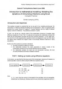
Queuing system diagram

Requestors

Server

issue

provides

Random variables

service request service request service request service request service request service request

Service

A random variable X is a function that assigns a real-number value to each outcome of an experiment Usually described by a probability Rdensity function f (x) x and a distribution function F (x) = −∞ f (u)du

Queue

f (x) tells how likely it is that X’s value will be near x. Note that f (x) can be > 1.

Server

Service

X has an exponential distribution with parameter λ if it has Density function f (x) = λe−λ x ; x≥0 Distribution function F (x) = 1 − e−λ x ; x ≥ 0

serviced requests



Probabilities: 6-sided die, exponential

Renewal Processes Consider a sequence of events which happen first at time T0 = 0, then keep happening at random intervals

0.4 1.4 0.35

probability function: uniform

probability function: exponential

1.2

0.3

The events occur at times Tn (n = 0, 1, ...; T0 = 0), and Sn = Tn − Tn−1 (n = 1, 2, ...) are the times between them, often called renewal periods

1

0.25

0.8

0.2 0.15

0.6

0.1

0.4

0.05

0.2

0

lambda = 1.0 lambda = 0.5 lambda = 0.25

0 0

1

2

3

4

5

6

7

8

0

1.6

1

2

3

4

5

6

7

If the random variables Sn are independent and identically distributed (iid), then the sequence {Tn ; n = 0, 1, ...} is a renewal process

1.4

distribution function: uniform

1.4

Renewal processes are useful for modelling streams of packets on a wire, jobs to be processed, etc.

distribution function: exponential

1.2

1.2

1

1 0.8

A renewal process is completely characterised by the common distribution function, F (x), or the density function, f (x) (if it exists), of its renewal periods

0.8 0.6 0.6 0.4

0.4

lambda = 1.0 lambda = 0.5 lambda = 0.25

0.2

0.2 0

0 0

1

2

3

4

5

6

7

8

0

1

2

3

4

5


Poisson processes (1)


Poisson processes (2)

A renewal process with exponentially distributed renewal periods S, i.e. F (x) = 1 − e−λ x , is called a Poisson process

Uniform arrival rate: P (S ≤ t + ∆t | S > t) ≈ λ ∆t, f or small ∆t

Poisson processes are often used in modelling. They derive several useful properties from the exponential distribution, as follows .. Lack of memory: P (S ≤ t + ∆t | S > t) = P (S ≤ t); s, t ≥ 0

Superposition:

Knowing that the process has been running for time t doesn’t affect its distribution for the remaining time (i.e. the time until the next event) The process forgets its past


With a Poisson process, arrivals occur at an average rate λ This implies PASTA: Poisson Arrivals See Time Averages A Poisson arrival acts as a random observer and sees the queue in equilibrium If A1 , A2 , ...An are independent Poisson processes with rates λ1 , λ2 , ...λn , their superposition is also a Poisson process, with rate λ1 + λ2 ... + λn A Poisson process can also be decomposed into a set of Poisson processes


Kendall notation of a queuing problem

Poisson distribution For a Poisson process, i.e. exponential distribution of interarrival times (renewal periods): Probability that n arrivals occur in interval of length t is n −λt Pn (t) = (λt) n! e This formula is the Poisson distribution with parameter λ t, for which M ean = λt, and V ar = λt λ is the mean rate, i.e. λ events occur per unit time

More generally . . . Mean of random variable X: R∞ M ean(X) = E[X] = −∞ x f (x)dx

Variance of X: V ar(X) = σ 2 = E[(X − E[X])2 ]

ArrDist/ServDist/Servers/Buffers/Population/ServDisc A queuing problem can be described by its arrival distribution (arrival times of service requests) service distribution (time server takes to service a request) number of available servers buffers (total number of possible service requests in the system) population (total number of possible requests) service discipline (in which order do we deal with requests?)

We often only give first three, e.g. M/M/1 other parameters take default values, i.e. ∞/∞/F IF O



Deterministic arrival distributions (D)

Arrival time distributions Need to model the arrival process (customers coming through bank door, packets arriving at router)

Very simple: All inter-arrival times τ are constant! τ = 1/λ

Some processes have highly predictable arrival processes (e.g., a plane lands and 100 passengers get off), others have a less deterministic nature (e.g., customers arriving at a bank) Arrival processes are renewal processes Can often model arrivals using statistical distributions e.g. (Kendall notation in parentheses),Exponential (M ), deterministic (D), Erlang with parameter k (Ek ) The thing we’re usually interested in is the interarrival time; average arrival rate (arrivals per time unit) is denoted as λ where applicable



Exponential arrival distributions (M )

Erlang arrival distributions (Ek )

Exponential arrival distributions are perhaps the most common apart from deterministic ones Approximately exponentially distributed, e.g. the time until you next meet a friend you haven’t heard from in 2 years, the time the next customer walks through the door at your local supermarket, etc. Rt Exponential distribution: P (S ≤ t) = 0 λ e−λu du S = time between two arrivals (random variable) Probability next arrival occurs in t seconds is P (S ≤ t).

Interarrival time probability given by Z t (λu)k−1 −λu P (S ≤ t) = λ e du (k − 1)! 0 Values ≥ 0, two parameters: M ean = 1/λ, shape k, – often more realistic than plain exponential Applies to a cascade of servers with exponential distribution times, such that a customer can’t be started until the previous one has been completely processed When k is integer, Erlang distribution is sum of k independent exponential distributions (gamma function)

Mean of S is 1/λ, standard deviation is also 1/λ. (Remember: λ is the mean arrival rate)

Note that the exponential distribution results for k = 1

Memoryless


Exponential and Erlang plots


Service time distributions Service time: time that a server needs to deal with a service request. For example, the time it takes to re-fuel a car or the time it takes to route a packet at a router Average service time is often denoted as 1/µ, where µ is the average service rate (number of requests serviced per time unit) per server Can model these service times via distributions – basically the same as for arrival time distributions. Just use µ instead of λ

P(S