Introduction to Scientific Programming Olaf Ippisch email:
[email protected] 30. Juli 2009
Inhaltsverzeichnis 1 Introduction 1.1 Subject of the Lecture . . . . . . . . . . . . . . . . . . . . . . . . . . . . . . . .
4 4
2 Repetition 2.1 Constants . . . . . . . . . . . . . . . . . . . . . . . . . . . . . . . . . . . . . . .
13 19
3 Number Representation in Computers
20
4 Repetition
22
5 Real Numbers
22
6 Round-off Errors
26
7 Conditioned Execution
26
8 Blocks
29
9 Functions 9.1 Mathematical Functions of the Standard Library . . . . . . . . . . . . . . . . . 9.2 Function Arguments . . . . . . . . . . . . . . . . . . . . . . . . . . . . . . . . .
29 29 31
10 Exercises
32
11 Functions 11.1 Local Variables . . . . . . . . . . . . . . . . . . . . . . . . . . . . . . . . . . . . 11.2 Call by Value and Call by Reference . . . . . . . . . . . . . . . . . . . . . . . . 11.3 Function Overloading . . . . . . . . . . . . . . . . . . . . . . . . . . . . . . . . .
35 35 36 38
12 Loops
40
13 Loops
46
14 Formatted IO
47
1
15 Comments
48
16 Runtime Measurement
49
17 Exercises
50
18 Arrays in C++
58
19 Solution of Linear Equation Systems
62
20 Self-defined Variable Types
65
21 Advantages of object-oriented programming
69
22 Object-oriented programming in C++
71
23 Classes
78
24 Direct Solution of Linear Equation Systems
80
25 Tridiagonal Matrices
81
26 Default Methods
85
27 Constant Objects
86
28 Operators
87
29 Example Improved Matrix Class
90
30 Preprocessor
96
31 Inheritance
97
32 Inheritance
98
33 Virtual Functions
100
34 Interface Base Classes
102
35 Interpolation 102 35.1 Interpolation with Polynomials . . . . . . . . . . . . . . . . . . . . . . . . . . . 102 35.2 Example . . . . . . . . . . . . . . . . . . . . . . . . . . . . . . . . . . . . . . . . 105 36 Namespaces
108
37 Makefiles
109
38 Streams
110
39 Homework
115
2
40 Homework
116
41 Generic Programming 41.1 Templates . . . . . . . . . . . . . . . . . . . . 41.2 Non-Numerical MatrixClass with Templates 41.3 Derived NumMatrixClass with Templates . . 41.4 Application of MatrixClass with Templates . 41.5 The Standard Template Library (STL) . . . . 42 Résumé
. . . . .
. . . . .
. . . . .
. . . . .
. . . . .
. . . . .
. . . . .
. . . . .
. . . . .
. . . . .
. . . . .
. . . . .
. . . . .
. . . . .
. . . . .
. . . . .
. . . . .
. . . . .
. . . . .
117 117 119 120 122 123 128
3
1 Introduction 1.1 Subject of the Lecture Intention of the Lecture • Other lectures cover theoretical or applied aspects of modeling and simulation (equations, material properties, mathematical aspects of partial differential equations, numerical methods) • In this lecture we will learn how to solve numerical problems with our own programs • To realize this we will need knowledge on – computer science – programming (C++) – numerical algorithms • In a second lecture (Advanced Scientific Programming) this knowledge is used to implement a (parallel) solver for a real problem (ground water flow, linear elasticity) Aims • Learn an industry standard programming language • Learn modern programming techniques • Get a better understanding for the solution of numerical problems with a computer and the limitations • Get an insight in the operation of simulation programs Prerequisites • Basic knowledge of numerical mathematics • Readiness to do the programming exercises Topics • Computer Science Basics • Programming – – – – – – –
Structure of C++ Programs Variables Input/Output Control Structures (Conditional Execution/Loops) Functions Arrays Containers
4
– – – –
Classes Inheritance Interfaces and Abstract Classes Generic Programming
Topics (ctd.) • Numerics – – – – –
Floating Point Numbers Interpolation Numerical Differentiation Numerical Integration Solution of Linear Equation Systems
Practical Exercises and Exam • Programming exercises each week (solution has to be presented by a student in the next lecture) • Three homeworks (have to be handed in) • 50 percent of the obtainable points necessary as a precondition for the final test • Written examination at the end of the Course Course Homepage The address of the course homepage is http://www.ipvs.uni-stuttgart.de/abteilungen/sgs/lehre/ lehrveranstaltungen/vorlesungen/WS0809/commasc6/en You will find there: • the transparencies shown in the lectures (after the lecture) • the exercises and homeworks • links to additional material and a list of suggested books • instructions how to get a C++ compiler COMMAS computer lab • The COMMAS computer lab is located in room 2.166 (just the next door) • The available computers are running Linux (OpenSUSE) • There is also a printer available • Linux is the default operating system for all COMMAS lectures • All the software necessary to do the exercises is already installed
5
How to solve a Problem with a Computer?
Program (on paper)
Problem Idea Work
Debugging
Algorithm doesn’t work too slow
works
Production
Algorithm • is a recipe for the solution of a problem • gives a sequence of steps to reach the target • has to be – precise – non-ambiguous – complete
6
Processor
– finite and composed of finite operations – correct • Example: Sort the names of the Commas-students Sort Names of COMMAS-Students Soyer, Ahmet Mert Raina, Arun Olivares Garcia, Cesar Fernando Gorne Zoppi, Christofer Elias Tunuguntala, Deepak Halit, Demir Naik, Dhavalnitinbabu Ramasamy, Ellankavi Rajabali, Fatemeh Gültekin, Furkan Al-Tameemi, Hamza A. Hussain Shah, Kaushal Aram, Maedeh Salman, Marwan A. Khalifa, Mohamed Abdel Salam, Mohamed Rani Rahman, Mohammad Tanvir Ahamed, Mohi Uddin Mahdi, Mottahedi Tkachuk, Mykola Pillai, Rachana Roshan, Rakesh Narizhnyy, Roman Kulkarni, Romit Ashok Sridhar, Sabari Nathan Patil, Sandeep Parasharam Ravipati, Satya Krishna Alizadeh Sabet, Sepideh Janwe, Snehal Pradeep Spreng, Stefan Vallabhuni, Tarun Dhanpal, Yogesh
What is a good Algorithm Generality Can the algorithm be applied to a wide variety of cases (e.g. an integration algorithm can integrate smooth and non-smooth functions or scalar and vector functions)? Complexity How does the numerical effort scale with the size N of the problem (e.g. the number of names to be sorted)? Sorting can be done e.g. by • selection sort (minimal amount of copy operations, no additional memory needed, but does not scale well, is O(N 2 )). • merge sort (needs twice the amount of memory, but is O(N ·ld(N )) which is optimal) Program • A program is used to describe an algorithm in a form, which can be understood by a computer What is the Computers Language? • The Central Processing Units of computers are complex arrays of switches • The machine language therefore consists of sequences of 0 and 1 (for 0 for off and 1 for on) • One digit of a machine code instruction is called bit • Several bits form an instruction word, which can be followed by one or more arguments • The CPU is capable of doing integer and floating point calculations and conditional execution. It can fetch instructions and values from the memory and write them to the memory • To facilitate program development assembler languages are used, which replace the machine code instruction sequences of 0 and 1 with instruction words (e.g. mov, add) • Each processor or processor family has its own machine language
7
Program • A program is used to describe an algorithm in a form, which can be understood by a computer • There is a huge variety of different programming languages due to historical and functional reasons. They differ in – – – – – – –
time necessary for the development of a program time necessary for the translation of the program into machine language execution speed of the final programs readability of the code amount of error checking done by the programming environment portability extensibility
High-level and low-level Programming Languages There are high-level and low-level programming languages. • Low-level languages are – – – –
very close to the machine language of a processor fast to translate and execute hard to read hard to port to other processor architectures
• High-level languages are – – – –
closer to human language easier to read and maintain better portable often slower than low-level languages
Faculty in x86-Assembler .globl factorial factorial: movl $1, %eax jmp .L2 .L3: imull 4(%esp), %eax decl 4(%esp) .L2: cmpl $1, 4(%esp) jg .L3 ret
in C++ int factorial (int n) { if (n==0) return 1; else return n*factorial(n-1); }
8
Compiler Languages and Interpreter Languages Programming languages either use a compiler or an interpreter to translate the program text into machine language. • An interpreter translates the program text command for command into machine language during each execution. This makes program execution slower, but the same program can easily be executed on different architectures, it can be executed immediately after it is written and can be changed during execution • A compiler translates the whole program text once into a binary executable file. This only has to be done once. The binary executable can only be used on one architecture. It executes faster, but during program development one always has to wait until the compiler has finished before the program can be tested. Faculty in Python
content of program file faculty.py
def factorial(n): if n == 0: return 1 else: return n*factorial(n-1) print factorial(10)
in C++
content of program file faculty.cc
#include int factorial (int n) { if (n==0) return 1; else return n*factorial(n-1); } int main () { std::cout


![[PDF] Introduction to Scientific Programming and ... - Google Sites](https://m.moam.info/img/260x300/pdf-introduction-to-scientific-programming-and-goo_647777a4097c474b228c1ba2.jpg)