Introduction to Speech Recognition
1
Paul R. Dixon Yandex Zurich
[email protected]
2 Overview of a Statistical Speech Recognition Training Data
Acoustic models
Spoken utterance
Feature extraction
¡ Statistical model built from large data and expert knowledge ¡ Language independent – Japanese, arabic, …
¡ Signal processing to extract salient features from speech
Pronunciation model
Language model
Search Written transcription
¡ Search – Given the models and audio input generate text transcription ¡ Voice search, dictation, transcription of meetings, talks and lectures, audio indexing + keyword spotting
3
P (Wn |Wn
N +1 , . . . , Wn 1 )
N
Speech Decoding Problem
Count(W1 , W2 , W3 P (W3 |W1 , W2 ) = Language Model Count(W 2 , W3 ) 9
𝑮
𝑳
10 N-grams
P (Wn |Wn
N +1 , . . . , Wn
106 Words
1) =
Count(Wn N +1 Count(Wn N + e
O ) = PI P (C3i |O 10
𝑯𝑪
𝑶
Phones 105 Gaussians
j=1
ai
e
aj
O) P (Ci |O O P (O |Ci )from = Acoustic score Search P (C ) i graph utterance W⇤ = Best(O H C L G) Best word sequence
Acoustic
1 Lexicon Grammar
Evaluation of Speech Recognition Hyp Ref Error
A A The Sub Ins
Dog Dog
Ate Ate
Homework My Homework Del (Example source: Kingsbury 2009)
Error types: Substitution, Deletion, Insertions Find best alignment with edit (Levenstein) distance Word Error Rate (WER) =
100 x number of errors number reference words
Real Time Factor (RTF) Task: Domain, vocabulary, Time taken / Length of speech language model size,…. Memory Usage Memory taken to store the Other metrics models and search usage Latency, Sentence Error Rate
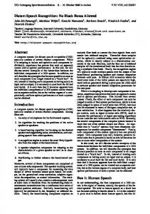
comprehensive series of tests on ASR over two and a half decades, and the performance of major ASR benchmark tests is summarized in [19]. Here we reproduce the results in Figure 1 for the readers’ reference.
Applications of this optimization framework to MT and the extension to ST will be presented in this lecture note. To conclude this brief introduction, we point out that in each of the ASR, MT, and ST fields, a series of benchmark evalua-
arning of ST systems. On the other hand, discriminative arning has been used pervasively in cent statistical signal processing and attern recognition research including SR and MT separately [7], [13], [26]. In
PR
Performance of Speech Recognition Conversational Speech
Switchboard
(Non-English)
Read Speech
Meeting Speech Meeting—SDMOV4 Meeting—MDMOV4
Switchboard II
EE
Broadcast Speech
Air Travel Planning Kiosk Speech
Varied Microphones
CTS Arabic (UL) CTS Mandarin (UL)0 Meeting—IHM News Mandarin 10X News Arabic 10X
(Non-English)
CTS Fisher (UL)
20k
Noisy
5k
Mismatches cause huge problems
News English 1X
News English Unlimited
10
News English 10X
IE
WER (%)
[Image source He & Deng 2011]
NIST STT Benchmark Test History—May 2009
100
1k
Stops before Deep Learning became popular
4
Range of Human Error in Transcription
2
2011
2010
2009
2008
2007
2000
2005
2004
2003
2002
2001
2000
1998
1998
1997
1996
1995
1994
1993
1992
1991
1990
1989
1988
1
IG1] After [19], a summarization of historical performance progresses on major ASR benchmark tests conducted by NIST.
Move on to more difficult tasks IEEE SIGNAL PROCESSING MAGAZINE [2] SEPTEMBER 2011
Conversational Telephone Speech (CTS)
Results
In Practice Tune for a Trade Moses Benchmarks: 8 Threads off38Between WER/RTF8 marks: Threads
2
Backoff Models Data Structures Results
Perplexity Translation
Rand Backoff 2≠8 false
4
29
8 Rand Backoff 2≠8 false
Time WER (h)
27
1 2
25
Chop
8
Chop
8
8
23
1 8 Trie 4 21 19
0
17
00
4
,
Trie
Probing
0.1
2
0.2
6 8 Memory (GB)
4
/
SRI Each curve represents a Probing different system
6 0.4 80.5 10 12 RTF Memory (GB) 0.3
Heafield
SRI
10
0.6
KenLM: Faster and Smaller Language Model Queries
Fundamental Equation of Speech Recognition Where: W |O O) W ⇤ = arg max P (W W
O |W W )P (W ) P (O = arg max O) P (O W O |W W )P (W W) = arg max P (O
W
⇡ arg m W
W some word sequence W ⇤ is the best word sequence O is a sequence of acoustic vectors
Bayes0 rule O ) is constant P (O
W
O |W W ) + log P (W W )} = arg max {log P (O
To avoid underflow
W
O |W W ) + ↵ log P (W W )} = arg max {log P (O W
Where: W some word sequence W ⇤Challenges: is the best word sequence is a sequence of acoustic vectors 1. Efficiently build accurate is the language model weight
models 2. Efficiently decode speech
Fudge factor
Formulate Recognition as a Transduction ¡ Weighted Finite State Transducers [Pereira 1994, Mohri 2009]give an formal framework for expressing the models providing operations: ¡ Composition: Combine levels of information ¡ Determinization: Optimize for speed
¡ Models are learned from data ¡ N-grams, Gaussian mixture models, (Hidden) Markov models, Neural networks
Sentence
Word
Phone
Acoustic
Weighted Finite State Transducers
¡ Generalization of a finite state machine ¡ Pioneered at AT&T in the mid 90s ¡ Weighted mapping between strings
¡ Unified framework for representation and optimization
¡ See OpenFst - http://openfst.org Input label
Output label
Weight
Initial state
Sentence
Final states
Word
Phone
Acoustic
Language Model ¡ Disambiguate acoustic similar words ¡ Recognize speech ¡ Wreck a nice beach
¡ Most popular model is a simple N-gram ¡ Easy to train and scales well
¡ Used in many tasks, POS tagging, machine translation, handwriting recognition, text prediction, sentiment analysis
Sentence
Word
Phone
Acoustic
: uence word sequence Language Model ic vectors best 2 word sequence Model weight ¡ Want Language to compute uence of acoustic vectors nguage model weight P (W 1 , W2 , W3 , . . . , Wn ) = P (W1 )P (W2 |W1 )P (W
Model ¡ Apply chain rule nguage P (W )P1(W (W = P (W1 )P (WModel (W13 |W , W22|W ) . .1. )P P (W . W(W 2 |W1 )P n |W 1 .2.)P n 14)|W 3 |W
, W3¡ , A . .pproximate . , Wn ) = P (W (W2 |W1 )P (W , W2 ) . . . P (Wn with history 1 )Ptruncated 3 |W1(Bigram) W1 )P (W3 |W2 )P (W4 |W3 ) . . . P (Wn |Wn 1 ) P (W1 )P (W2 |W1 )P (W3 |W2 )P (W4 |W3 ) . . . P (Wn |Wn Unigram
P (W1 )
Bigram
Unigram
1)
2
1
P (W3 |W1 , W2 )
Trigram
Count(W 1 , W2 , W3 ) N-gram Language Model P (W |W , . . . , W ) +1 n 1 P (W3 |W1n, Wn2 )N=
Count(W 2, W 3) ¡ Estimate parameters using Maximum likelihood Count(W W2 , W3 ) 1,) Count(W , W P (W3 |W1 , W2 ) = 1 2 P (W2 |W1 ) = Count(W2 , W3 ) Count(W1 )
P (Wn |Wn
Count(Wn N +1 , . . . , Wn ) N +1 , . . . , Wn 1 ) = Count(W . ., W . ,nW1n) ) Count(W n Nn+1 N,+1
n N +1 , . . . , Wn 1 )
=
Count(Wn e
O ) =/2.7081 P (Ci |O PI
j=1
/4.1997
ai
e
B/0.75869
/99 A/0.6799 aj
A/0.57053 A/0.82768
/99
O) P (Ci |O O |Ci ) = P (O P (Ci ) A/0.69415
N +1 , Wn 1 )
B/0.85175
A/2.9266
B/0.96444
B/0.69415
1 ¡ (In practice also use back-off, smoothing ……)
1
B/2.3575
Pronunciation Model ¡ Data sparsity means many words will never be seen or hardly seen ¡ Build words from smaller phoneme units ¡ Can recognize words not seen in training ¡ One of the few parts of the system that uses expert knowledge
Phoneme label
DH:THE DH:THE 0
Word label
Sentence
D:DOOR D:DOG
4
6
1
AH:
3
IY:
AO:
AO:
5
Epsilon/null transitions don’t consume symbols
R: G:
2
7
:
Word
Phone
Acoustic
Combining the Language Models and Lexicon DH:THE DH:THE 0
D:DOOR D:DOG
4
6
1
AH:
3
IY:
AO:
AO:
5
R: G:
0
2
THE
1
DOOR DOG
2
7
:
¡ Composition DH:THE 0
1
DH:THE
D:DOG
AH: IY:
3
:
4
5
7
G: R:
D:DOOR 6
2
AO:
AO:
9
8
¡ Determinization 0
DH:THE
1
AH: IY:
2
:
3
D:
4
AO:
5
G:DOG R:DOOR
6
Phone Model ¡ Hidden Markov models (HMMs) are the building block of modern ASR systems ¡ Typically a three state Hidden Markov ¡ Enforce a minimum phone durations
¡ Trained with expectation maximization algorithm ¡ In practice build context dependent units 2322/0.33423 0
1036/0.19008
2322/1.2584
1
PDF Index or DNN output unit
Sentence
510/0.29304
1036/1.7538
2
510/1.3704
Transition Probability (-log)
Word
Phone
Acoustic
3
nd combined to give the overall probability of the vector under the
Acoustic p (xModeling | Q) = Â w p (x | ✓ )with Gaussian (2.1) Models is aMixtures data vector; the mixing parameters w are constrained so that 0 w 1 k
k k
k
k
k
wk = 1, ✓k represents the parameters of the k th Gaussian, and Q is used te all of the parameters in the model. Each component is a d dimensional p (x | Q ) = wk pk (x | ✓k ) (2.1) riate Gaussian density: k ⇢ 1 1 p x | ✓ = exp (x µk )T Sk 1 (x so µkthat ) (2.2) ( ) k parameters k he mixing w are constrained 0 wk 1 1/2 k d/2 2 (2p ) |Sk |
Â
sents the parameters of the k th Gaussian, and Q is used µk and Sk are the mean and covariances. The architecture of a GMM is shown meters in the model. Each component is a d dimensional work diagram in figure 2.1 . with expectation sity: ion ¡ Train from a GMM is simple. First a Gaussian component is chosen according to maximization algorithm r probabilities w = (w1 , w2⇢ , . . . , wk ), then a sample is drawn from the selected 1 n distribution. 1 1 T ¡ Speaker 1 adaptation exp ( x µ ) S ( x µ ) (2.2) k k ¡ Training can be k 1/2 2 and bootstrapping is 2p )d/2 S | | k parallelized Training a Gaussian Mixture Model straightforward mean covariances. architecture of a GMM is shown set¡ Scales ofand training data X = {xThe with data 1 , x2 , . . . , x N } drawn from an Independent lly Distributed learning process in involves gure 2.1 . (IID) probability distribution theImplementation http://kaldi.sf.net g the free parameters Q = w, µ, S (where all the individual weights, means, ( ) ¡ Speed up techniques ariances are grouped into acomponent tuple) to find theisMaximum s simple. First a together Gaussian chosenLikelihood according to Phone Acoustic =ughout (w1this , Sentence wthesis , then aWord sample from the selected willk ) denote probability mass and is p( x )drawn probability density function. In 2 , . P. (.x,) w
Count(W2 , W3
CD-DNN-HMM 2322/0.33423 0
Count(W1 , W2 , W P (W3 |W1 , W2 ) = Count(Wn N P (Wn |Wn N +1 , . . . , Wn 1 ) =Count(W2 , W3 )
1036/0.19008
2322/1.2584
O1 Ouput layer
H1
Hidden layer
1036/1.7538
1
.. . .. .
Input layer I1
I2
510/0.29304
I3
2
e Count(W n
O ) = PI P (Ci |O
j=1aie
On
e
aj
¡ Normalize priors O ) =byPstate P (Ci |O I to give HMM state Oaj) Pj=1 (Cei |O likelihoods O |Ci ) = P (O
P (C Oi )) P (C i |O O |Ci ) = P (O P (Ci )
Hn
.. .
P (W 510/1.3704 n |Wn 3
¡ Last layer has unit for Count(W n each HMM state Count(Wn N + softmax ai N +1 , . . . , Wn 1 ) =
¡ Trained with Stochastic Gradient Descent
1
In
¡ Input is a windows of 1 features ¡ Bootstrapped from a GMM system Implementation in http://kaldi.sf.net
N
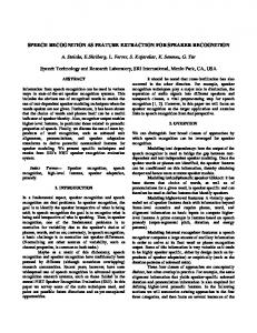
Performance of DNNs on Switchboard 300hrs task One-pass
Multi-pass / combination
Year
GMM
DNN
GMM
DNN
Details
2011
23.6
16.1
17.1
-
(Seide 2011)
2012
18.9
13.3
15.1
-
(Kingsbury 2012). DNN Sequence training
2013
18.6
12.6
-
(Vesely 2013). DNN Sequence training [^]
10.7
(Sainath 2014). Convolutional neural network
2014
11.5
14.5
(Disclaimer: potential differences in the experimental setups of the systems)
Search Algorithm ¡ Shortest path through a huge graph ¡ Dynamic programming ¡ Viterbi algorithm ¡ Beam search ¡ At any time, only keep the states that are within a given beam of the best scoring state
Open Source Resources (not exhaustive) Kaldi - http://kaldi.sourceforge.net OpenFst - http://openfst.org OpenGrm - http://opengrm.org Phonetisaurus - https://code.google.com/p/phonetisaurus/ Voxforge http://http://voxforge.org/ TED LIUM corpus http://www-lium.univ-lemans.fr/en/content/ted-lium-corpus CMU dictionary http://www.speech.cs.cmu.edu/cgi-bin/cmudict 1 Billion word benchmark https://code.google.com/p/1-billion-word-language-modelingbenchmark/
Thanks for listening Questions?
References ¡ Xiaodong He and Li Deng, Speech Recognition, Machine Translation, and Speech Translation – A Unified Discriminative Learning Paradigm, in IEEE Signal Processing Magazine, September 2011 ¡ Jurafsky, Daniel, and James H. Martin. 2009. Speech and Language Processing: AnIntroduction to Natural Language Processing, Speech Recognition, and Computational Linguistics. 2nd edition ¡ Weighted Rational Transductions and their Application to Human Language Processing Fernando Pereira, Michael Riley, Richard W. Sproat Human Language Technology Workshop pp. 262-267 ¡ Mehryar Mohri. Weighted automata algorithms. 2009. ¡ Frank Seide, Gang Li, and Dong Yu, Conversational Speech Transcription Using Context-Dependent Deep Neural Networks, in Interspeech 2011 ¡ B. Kingsbury, T. N. Sainath, and H. Soltau, “Scalable minimum Bayes risk training of deep neural network acoustic models using distributed Hessian-free optimization,” in Proc. INTERSPEECH, September 2012 ¡ "Sequence-discriminative training of deep neural networks", K. Vesely, A. Ghoshal, L. Burget and D. Povey, Interspeech 2013 ¡ Tara N. Sainath Improvements to Deep Neural Networks for Large Vocabulary Continuous Speech Recognition Tasks 2014 http://wissap.iiit.ac.in/proceedings/ TSai_L8.pdf
ASR and Speech Processing ¡ Automatic Speech Recognition (ASR)
¡ Given a audio input – generate text transcription ¡ Applications: voice search, dictation, transcription of meetings, talks and lectures, audio indexing + keyword spotting
¡ Speech synthesis – text to speech
¡ Voice conversion, singing synthesis
¡ Speaker recognition
¡ Speaker verification - Speaker identification ¡ Related tasks, gender or language
¡ Spoken dialogue/understanding systems, speech enhancement ¡ Machine translation
What Makes Speech Recognition Hard? Speaker
Environment
• Age • Accent/ Dialect/Nonnative • Speaking rate • Co-articulation • Style • Physical differences • Language
• Background noise • Other speakers • Reverberation • Microphone placement
Audio quality • Device • Channel characteristics • Knowledge of the task • Volume
Changes and variations in conditions will often cause a huge impact on recognition performance
The Noisy Channel Model Noisy Channel Model
(Image source Jurafsky & Martin 2009)
! Search through space of all possible sentences. ¡ Acoustic realization is a corrupted ¡ Statistical speech processing ! Pickofthe one that is most probable given ¡ CMU Harpy and the IBM 1970s version the original text waveform.
¡ Same framework for many problems including: OCR ¡ Build a channel model so we can recognition, machine recover the original translation ¡ Passed through a noisy channel