Oct 5, 2008 ... Introduction to Stata. CEP and STICERD. London School of Economics. Lent
Term 2009 ... WHAT STATA LOOKS LIKE . ..... Browse/Edit .
Introduction to Stata
CEP and STICERD London School of Economics Lent Term 2009
Alexander C. Lembcke eMail:
[email protected] Homepage: http://personal.lse.ac.uk/lembcke
This is an updated version of Michal McMahon’s Stata notes. He taught this course at the Bank of England (2008) and at the LSE (2006, 2007). It builds on earlier courses given by Martin Stewart (2004) and Holger Breinlich (2005). Any errors are my sole responsibility. Page 1 of 61
Full Table of contents GETTING TO KNOW STATA AND GETTING STARTED ................................................................................. 5 WHY STATA? ............................................................................................................................................................. 5 WHAT STATA LOOKS LIKE ......................................................................................................................................... 5 DATA IN STATA.......................................................................................................................................................... 6 GETTING HELP............................................................................................................................................................ 7 Manuals ................................................................................................................................................................ 7 Stata’s in-built help and website .......................................................................................................................... 7 The web................................................................................................................................................................. 7 Colleagues ............................................................................................................................................................ 7 Textbooks .............................................................................................................................................................. 7 DIRECTORIES AND FOLDERS ....................................................................................................................................... 8 READING DATA INTO STATA ...................................................................................................................................... 8 use......................................................................................................................................................................... 8 insheet................................................................................................................................................................... 8 infix ....................................................................................................................................................................... 9 Stat/Transfer program ........................................................................................................................................ 10 Manual typing or copy-and-paste....................................................................................................................... 10 VARIABLE AND DATA TYPES .................................................................................................................................... 11 Indicator or data variables ................................................................................................................................. 11 Numeric or string data ....................................................................................................................................... 11 Missing values .................................................................................................................................................... 11 EXAMINING THE DATA ............................................................................................................................................. 12 List ...................................................................................................................................................................... 12 Subsetting the data (if and in qualifiers) ............................................................................................................ 12 Browse/Edit ........................................................................................................................................................ 13 Assert .................................................................................................................................................................. 13 Describe.............................................................................................................................................................. 13 Codebook ............................................................................................................................................................ 13 Summarize .......................................................................................................................................................... 13 Tabulate .............................................................................................................................................................. 14 Inspect ................................................................................................................................................................ 15 Graph ................................................................................................................................................................. 15 SAVING THE DATASET .............................................................................................................................................. 15 Preserve and restore ........................................................................................................................................... 15 KEEPING TRACK OF THINGS ...................................................................................................................................... 16 Do-files and log-files .......................................................................................................................................... 16 Labels ................................................................................................................................................................. 17 Notes ................................................................................................................................................................... 18 Review ................................................................................................................................................................ 18 SOME SHORTCUTS FOR WORKING WITH STATA ........................................................................................................ 19 A NOTE ON WORKING EMPIRICAL PROJECTS. ............................................................................................................ 19 DATABASE MANIPULATION ............................................................................................................................... 20 ORGANISING DATASETS ........................................................................................................................................... 20 Rename ............................................................................................................................................................... 20 Recode and replace ............................................................................................................................................ 20 Mvdecode and mvencode .................................................................................................................................... 20 Keep and drop (including some further notes on if-processing) ........................................................................ 20 Sort ..................................................................................................................................................................... 22 By-processing ..................................................................................................................................................... 23 Append, merge and joinby .................................................................................................................................. 23 Collapse .............................................................................................................................................................. 25 Order, aorder, and move .................................................................................................................................... 25 CREATING NEW VARIABLES ..................................................................................................................................... 26 Generate, egen, replace ...................................................................................................................................... 26 Converting strings to numerics and vice versa ................................................................................................... 26 Page 2 of 61
Combining and dividing variables...................................................................................................................... 27 Dummy variables ................................................................................................................................................ 28 Lags and leads .................................................................................................................................................... 29 CLEANING THE DATA ............................................................................................................................................... 30 Fillin and expand................................................................................................................................................ 30 Interpolation and extrapolation .......................................................................................................................... 30 Splicing data from an additional source ............................................................................................................ 31 PANEL DATA MANIPULATION: LONG VERSUS WIDE DATA SETS .............................................................................. 31 Reshape .............................................................................................................................................................. 32 ESTIMATION............................................................................................................................................................ 34 DESCRIPTIVE GRAPHS .............................................................................................................................................. 34 ESTIMATION SYNTAX ............................................................................................................................................... 37 WEIGHTS AND SUBSETS............................................................................................................................................ 37 LINEAR REGRESSION ................................................................................................................................................ 38 POST-ESTIMATION .................................................................................................................................................... 41 Prediction ........................................................................................................................................................... 41 Hypothesis testing ............................................................................................................................................... 41 Extracting results................................................................................................................................................ 43 OUTREG2 – the ultimate tool in Stata/Latex or Word friendliness? ................................................................. 44 EXTRA COMMANDS ON THE NET ............................................................................................................................... 45 Looking for specific commands .......................................................................................................................... 45 Checking for updates in general ......................................................................................................................... 46 Problems when installing additional commands on shared PCs ........................................................................ 47 Exporting results “by hand” .............................................................................................................................. 48 CONSTRAINED LINEAR REGRESSION ......................................................................................................................... 50 DICHOTOMOUS DEPENDENT VARIABLE .................................................................................................................... 50 PANEL DATA ............................................................................................................................................................ 51 Describe pattern of xt data ................................................................................................................................. 51 Summarize xt data .............................................................................................................................................. 52 Tabulate xt data .................................................................................................................................................. 53 Panel regressions ............................................................................................................................................... 53 TIME SERIES DATA ................................................................................................................................................... 56 Stata Date and Time-series Variables ................................................................................................................ 56 Getting dates into Stata format ........................................................................................................................... 57 Using the time series date variables ................................................................................................................... 58 Making use of Dates ........................................................................................................................................... 59 Time-series tricks using Dates ............................................................................................................................ 59 SURVEY DATA .......................................................................................................................................................... 61
Page 3 of 61
Course Outline This course is run over 8 weeks during this time it is not possible to cover everything – it never is with a program as large and as flexible as Stata. Therefore, I shall endeavour to take you from a position of complete novice (some having never seen the program before), to a position from which you are confident users who, through practice, can become intermediate and onto expert users. In order to help you, the course is based around practical examples – these examples use macro data but have no economic meaning to them. They are simply there to show you how the program works. There will be some optional exercises, for which data is provided on my website – http://personal.lse.ac.uk/lembcke. These are to be completed in your own time, there should be some time at the end of each meeting where you can play around with Stata yourself and ask specific questions. The course will follow the layout of this handout and the plan is to cover the following topics. Week
Time/Place
Activity
Week 1
Tue, 17:30 – 19:30 (S169)
Getting started with Stata
Week 2
Tue, 17:30 – 19:30 (S169)
Database Manipulation and graphs
Week 3
Tue, 17:30 – 19:30 (S169)
More database manipulation, regression and post-regression analysis
Week 4
Tue, 17:30 – 19:30 (S169)
Advanced estimation methods in Stata
Week 5
Tue, 17:30 – 19:30 (S169)
Programming basics in Stata
Week 6
Tue, 17:30 – 19:30 (S169)
Writing Stata programs
Week 7
Tue, 17:30 – 19:30 (S169)
Mata
Week 8
Tue, 17:30 – 19:30 (S169)
Maximum Likelihood Methods in Stata
I am very flexible about the actual classes, and I am happy to move at the pace desired by the participants. But if there is anything specific that you wish you to ask me, or material that you would like to see covered in greater detail, I am happy to accommodate these requests.
Page 4 of 61
Getting to Know Stata and Getting Started Why Stata? There are lots of people who use Stata for their applied econometrics work. But there are also numerous people who use other packages (SPSS, Eviews or Microfit for those getting started, RATS/CATS for the time series specialists, or R, Matlab, Gauss, or Fortran for the really hardcore). So the first question that you should ask yourself is why should I use Stata? Stata is an integrated statistical analysis packaged designed for research professionals. The official website is http://www.stata.com/. Its main strengths are handling and manipulating large data sets (e.g. millions of observations!), and it has ever-growing capabilities for handling panel and time-series regression analysis. The most recent version is Stata 10 and with each version there are improvements in computing speed, capabilities and functionality. It now also has pretty flexible graphics capabilities. It is also constantly being updated or advanced by users with a specific need – this means that even if a particular regression approach is not a standard feature, you can usually find someone on the web who has written a programme to carry-out the analysis and this is easily integrated with your own software.
What Stata looks like On LSE computers the Stata package is located on a software server and can be started by either going through the Start menu (Start – Programs – Statistics – Stata10) or by double clicking on wsestata.exe in the W:\Stata10 folder. The current version is Stata 10. In the research centres the package is also on a server (\\st-server5\stata10$), but you should be able to start Stata either from the quick launch toolbar or by going through Start – Programs.
There are 4 different packages available: Stata MP (multi-processor) which is the most powerful, Stata SE (special edition), Intercooled STATA and Small STATA. The main difference between these versions is the maximum number of variables, regressors and observations that can be handled (see http://www.stata.com/order/options-e.html#difference-sm for details). The LSE is currently running the SE-version, version 10. Stata is a command-driven package. Although the newest versions also have pull-down menus from which different commands can be chosen, the best way to learn Stata is still by typing in the commands. This has the advantage of making the switch to programming much easier which will be necessary for any serious econometric work. However, sometimes the exact syntax of a command is hard to get right –in these cases, I often use the menu-commands to do it once and then copy the syntax that appears.
Page 5 of 61
You can enter commands in either of three ways: -
Interactively: you click through the menu on top of the screen Manually: you type the first command in the command window and execute it, then the next, and so on. Do-file: type up a list of commands in a “do-file”, essentially a computer programme, and execute the do-file.
The vast majority of your work should use do-files. If you have a long list of commands, executing a do-file once is a lot quicker than executing several commands one after another. Furthermore, the do-file is a permanent record of all your commands and the order in which you ran them. This is useful if you need to “tweak” things or correct mistakes – instead of inputting all the commands again one after another, just amend the do-file and re-run it. Working interactively is useful for “I wonder what happens if …?” situations. When you find out what happens, you can then add the appropriate command to your do-file. To start with we’ll work interactively, and once you get the hang of that we will move on to do-files.
Functions
Variables
Interactive (Menus)
Stata Mata User written
Command window
Output
Do/Ado - Files Save/Export
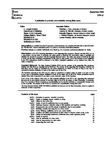
Data in Stata Stata is a versatile program that can read several different types of data. Mainly files in its own dta format, but also raw data saved in plain text format (ASCII format). Every program you use (i.e. Excel or other statistical packages) will allow you to export your data in some kind of ASCII file. So you should be able to load all data into Stata. When you enter the data in Stata it will be in the form of variables. Variables are organized as column vectors with individual observations in each row. They can hold numeric data as well as strings. Each row is associated with one observation, that is the 5th row in each variable holds the information of the 5th individual, country, firm or whatever information you data entails. Information in Stata is usually and most efficiently stored in variables. But in some cases it might be easier to use other forms of storage. The other two forms of storage you might find useful are matrices and macros. Matrices have rows and columns that are not associated with any observations. You can for example store an estimated coefficient vector as a k × 1 matrix (i.e. a column vector) or the variance matrix which is k × k. Matrices use more memory then variables and the size of matrices is limited 11,000 (800 in Stata/IC), but your memory will probably run out before you hit that limit. You should therefore use matrices sparingly. The third option you have is to use macros. Macros are in Stata what variables are in other programming languages, i.e. named containers for information of any kind. Macros come in two different flavours, local or temporary and global. Global macros stay in the system and once set, can be accessed by all your commands. Local macros and temporary objects are only created within a certain environment and only exist within that environment. If you use a local macro in a do-file it, you can only use it for code within that do-file.
Data
Stata
Stata: dta Excel: xls, csv Ascii: csv, dat, txt etc… Variables
Text: string Numbers: integer double byte
Macros global local tempvar/name/file
Matrices
matrix vector scalar
Page 6 of 61
Getting help Stata is a command driven language – there are over 500 different commands and each has a particular syntax required to get any various options. Learning these commands is a time-consuming process but it is not hard. At the end of each class notes I shall try to list the commands that we have covered but there is no way we will cover all of them in this short introductory course. Luckily though, Stata has a fantastic options for getting help. In fact, most of your learning to use Stata will take the form of self-teaching by using manuals, the web, colleagues and Stata’s own help function.
Manuals The Stata manuals are available in LSE library as well as in different sections of the research centres. – many people have them on their desks. The User Manual provides an overall view on using Stata. There are also a number of Reference Volumes, which are basically encyclopaedias of all the different commands and all you ever needed to know about each one. If you want to find information on a particular command or a particular econometric technique, you should first look up the index at the back of any manual to find which volumes have the relevant information. Finally, there are several separate manuals for special topics such as a Graphics Manual, a panel data manual (cross-sectional time-series) or one on survey data.
Stata’s in-built help and website Stata also has an abbreviated version of its manuals built-in. Click on Help, then Contents. Stata’s website has a very useful FAQ section at http://www.stata.com/support/faqs/. Both the in-built help and the FAQs can be simultaneously searched from within Stata itself (see menu Help>Search). Stata’s website also has a list of helpful links at http://www.stata.com/links/resources1.html.
The web As with everything nowadays, the web is a great place to look to resolve problems. There are numerous chat-rooms about Stata commands, and plenty of authors put new programmes on their websites. Google should help you here.
Colleagues The other place where you can learn a lot is from speaking to colleagues who are more familiar with Stata functions than you are – the LSE is littered with people who spend large parts of their days typing different commands into Stata, you should make use of them if you get really stuck.
Textbooks There are some textbooks that offer an applied introduction to statistical or econometric topics using Stata. A basic textbook is “An Introduction to Modern Econometrics using Stata” by Christopher F. Baum. Who has also a book on programming in Stata “An Introduction to Stata Programming” forthcoming. A more advanced text is “Microeconometrics using Stata” by A. Colin Cameron and Pravin K. Trivedi, which will become available in the UK shortly. The last part of this book is based on William Gould, Jeffrey Pitblado, and William Sribney “Maximum Likelihood Estimation with Stata”, a book focussing solely on the Stata ml command.
Page 7 of 61
Directories and folders Like Dos, Linux, Unix and Windows, Stata can organise files in a tree-style directory with different folders. You should use this to organise your work in order to make it easier to find things at a later date. For example, create a folder “data” to hold all the datasets you use, sub-folders for each dataset, and so on. You can use some Dos and Linux/Unix commands in Stata, including: . . . .
cd “H:\ECStata” mkdir “FirstSession” dir pwd
-
change directory to “H:\ECStata” creates a new directory within the current one (here, H:\ECStata) list contents of directory or folder (you can also use the linux/unix command: ls) displays the current directory
Note, Stata is case sensitive, so it will not recognise the command CD or Cd. Also, quotes are only needed if the directory or folder name has spaces in it – “H:\temp\first folder” – but it’s a good habit to use them all the time. Another aspect you want to consider is whether you use absolute or relative file paths when working with Stata. Absolute file paths include the complete address of a file or folder. The cd command in the previous example is followed by an absolute path. The relative file path on the other hand gives the location of a file or folder relative to the folder that you are currently working in. In the previous example mkdir is followed by a relative path. We could have equivalently typed: . mkdir “H:\ECStata\FirstSession” Using relative paths is advantageous if you are working on different computers (i.e. your PC at home and a library PC or a server). This is important when you work on a larger or co-authored project, a topic we will come back to when considering project management. Also note that while Windows and Dos use a backslash “\” to separate folders, Linux and Unix use a slash “/”. This will give you trouble if you work with Stata on a server (ARC at the LSE). Since Windows is able to understand a slash as a separator, I suggest that you use slashes instead of backslashes when working with relative paths. . mkdir “/FirstSession/Data”
- create a directory “Data” in the folder H:\ECStata\FirstSession
Reading data into Stata When you read data into Stata what happens is that Stata puts a copy of the data into the memory (RAM) of your PC. All changes you make to the data are only temporary, i.e. they will be lost once you close Stata, unless you save the data. Since all analysis is contacted within the limitations of the memory, this is usually the bottle neck when working with large data sets. There are different ways of reading or entering data into Stata:
use If your data is in Stata format, then simply read it in as follows: . use "H:\ECStata\G7 less Germany pwt 90-2000.dta", clear The clear option will clear the revised dataset currently in memory before opening the other one. Or if you changed the directory already, the command can exclude the directory mapping:
. use "G7 less Germany pwt 90-2000.dta", clear If you are do not need all the variables from a data set, you can also load only some of the variables from a file.
. use country year using "G7 less Germany pwt 90-2000.dta", clear insheet If your data is originally in Excel or some other format, you need to prepare the data before reading it directly into Stata. You need to save the data in the other package (e.g. Excel) as either a csv (comma separated values ASCII text) or txt (tab-delimited ASCII text) file. There are some ground-rules to be followed when saving a csv- or txt-file for reading into Stata: -
The first line in the spreadsheet should have the variable names, e.g. series/code/name, and the second line onwards should have the data. If the top row of the file contains a title then delete this row before saving. Any extra lines below the data or to the right of the data (e.g. footnotes) will also be read in by Stata, so make sure that only the data itself is in the spreadsheet before saving. If necessary, select all the bottom rows and/or right-hand columns and Page 8 of 61
-
-
-
delete them. The variable names cannot begin with a number. If the file is laid out with years (e.g. 1980, 1985, 1990, 1995) on the top line, then Stata will run into problems. In such instances you can for example, place an underscore in front of each number (e.g. select the row and use the spreadsheet package’s “find and replace” tools): 1980 becomes _1980 and so on. Make sure there are no commas in the data as it will confuse Stata about where rows and columns start and finish (again, use “find and replace” to delete any commas before saving – you can select the entire worksheet in Excel by clicking on the empty box in the top-left corner, just above 1 and to the left of A). Some notations for missing values can confuse Stata, e.g. it will read double dots (..) or hyphens (-) as text. Use find & replace to replace such symbols with single dots (.) or simply to delete them altogether.
Once the csv- or txt-file is saved, you then read it into Stata using the command: . insheet using "H:\ECStata\G7 less Germany pwt 90-2000.txt", clear Note that if we had already changed to H:\ECStata using the cd command, we could simply type: . insheet using "G7 less Germany pwt 90-2000.txt", clear There are a few useful options for the insheet command (“options” in Stata are additional features of standard commands, usually appended after the command and separated by a comma – we will see many more of these). The first option is clear which you can use if you want to insheet a new file while there is still data in memory: . insheet using "H:\ECStata\G7 less Germany pwt 90-2000.txt", clear Alternatively, you could first erase the data in memory using the command clear and then insheet as before. The second option, names, tells Stata that the file you insheet contains the variable names in the first row. Normally, Stata should recognise this itself but sometimes it simply doesn’t – in these cases names forces Stata to use the first line in your data for variable names: . insheet using "F:\Stata classes\G7 less Germany pwt 90-2000.txt", names clear Finally, the option delimiter(“char”) tells Stata which delimiter is used in the data you want to insheet. Stata’s insheet automatically recognises tab- and comma-delimited data but sometimes different delimiters are used in datasets (such as “;”): . insheet using “h:\wdi-sample.txt”, delimiter(“;”)
infix While comma separated or tab delimited data is very common today, older data is often saved in a fixed ASCII format. The data cannot be read directly but a codebook is necessary that explains how the data is stored. An example for data that is stored this way is the U.S. National Health Interview Survey (NHIS). The first two lines of one of the 1986 wave look like this: 10861096028901 10861096028902
05 011 1 02130103000000000000000000001 05 011 1 02140103000000000000000000001
The codebook (usually a pdf or txt file) that accompanies the data tells you that the first 2 numbers code the record type, the following 2 numbers are the survey year (here 1986), the fifth number is the quarter (here the first quarter) of the interview and so on. To read this type of data into Stata we need to use the infix command and provide Stata with the information from the codebook. . infix rectype 1-2 year 3-4 quarter 5 […] using “H:\ECStata\NHIS1986.dat”, clear Since there are a lot of files it my be more convenient to save the codebook information in a separate file, a so called “dictionary file”. The file would look like this: infix dictionary using NHIS1986.dat { rectype 1-2 year 3-4 quarter 5 […] } Page 9 of 61
After setting up this file we would save it as NHIS1986.dct and use it in the infix command. Note that we used a relative path in the dictionary file, i.e. by not stating a file path for NHIS1986.dat we assume that the raw data is located in the same directory as the dictionary file. With the dictionary file we do not need to refer to the data directly anymore: . infix using “H:\ECStata\NHIS1986.dct”, clear Since setting up dictionary files is a lot of work, we are lucky that for the NHIS there exists already a dictionary file that can be read with SAS (a program similar to Stata). After reading the data into SAS and saving it we can use a tool called Stat/Transfer to convert the file into the Stata data format.
Stat/Transfer program This is a separate package that can be used to convert a variety of different file-types into other formats, e.g. SAS or Excel into Stata or vice versa. You should take great care to examine the converted data thoroughly to ensure it was converted properly. It is used in a very user-friendly way (see screen shot below) and is useful for changing data between lots of different packages and format.
Manual typing or copy-and-paste If you can open the data in Excel, you can usually copy and paste the data into the Stata data editor. All you need to do is select the columns in Excel; copy them; open the Stata data editor; and paste. This works usually quite well but entails certain pitfalls. The data format might not turn out to be correct, missing values might not be accounted for properly and in some cases language issues might arise (in some countries a comma rather than a decimal point is used). Manually typing in the data is the tedious last resort – if the data is not available in electronic format, you may have to type it in manually. Start the Stata program and use the edit command – this brings up a spreadsheet-like where you can enter new data or edit existing data. This can be done directly by typing the variables into the window, or indirectly using the input command.
Page 10 of 61
Variable and data types Indicator or data variables You can see the contents of a data file using the browse or edit command. The underlying numbers are stored in “data variables”, e.g. the cgdp variable contains national income data and the pop variable contains population data. To know what each data-point refers to, you also need at least one “indicator variable”, in our case countryisocode (or country) and year tell us what country and year each particular gdp and population figure refers to. The data might then look as follows: country
countryisocode
year
pop
cgdp
openc
Canada France Italy Japan United Kingdom United States
CAN FRA ITA JPN GBR USA
1990 1990 1990 1990 1990 1990
27700.9 58026.1 56719.2 123540 57561 249981
19653.69 17402.55 16817.21 19431.34 15930.71 23004.95
51.87665 43.46339 39.44491 19.81217 50.62695 20.61974
This layout ensures that each data-point is on a different row, which is necessary to make Stata commands work properly.
Numeric or string data Stata stores or formats data in either of two ways – numeric or string. Numeric will store numbers while string will store text (it can also be used to store numbers, but you will not be able to perform numerical analysis on those numbers). Numeric storage can be a bit complicated. Underneath its Windows platform, Stata, like any computer program, stores numbers in binary format using 1’s and 0’s. Binary numbers tend to take up a lot of space, so Stata will try to store the data in a more compact format. The different formats or storage types are: byte : integer between -127 and 100 e.g. dummy variable int : integer between -32,767 and 32,740 e.g. year variable long : integer between -2,147,483,647 and 2,147,483,620 e.g. population data float : real number with about 8 digits of accuracy e.g. production output data double : real number with about 16 digits of accuracy The Stata default is “float”, and this is accurate enough for most work. However, for critical work you should make sure that your data is “double”. Note, making all your numerical variables “double” can be used as an insurance policy against inaccuracy, but with large data-files this strategy can make the file very unwieldy – it can take up lots of hard-disk space and can slow down the running of Stata. Also, if space is at a premium, you should store integer variables as “byte” or “int”, where appropriate. The largest 27 numbers of each numeric format are reserved for missing values. For byte the standard missing value is 101, which will be represented by a dot (.) in Stata. Later when we evaluate logic expressions we need to account for this. String is arguably more straightforward – any variable can be designated as a string variable and can contain up to 244 characters, e.g. the variable name contains the names of the different countries. Sometimes, you might want to store numeric variables as strings, too. For example, your dataset might contain an indicator variable id which takes on 9-digit values. If id were stored in float format (which is accurate up to only 8 digits), you may encounter situations where different id codes are rounded to the same amount. Since we do not perform any calculations on id we could just as well store it in string format and avoid such problems. To preserve space, only store a variable with the minimum string necessary – so the longest named name is “United Kingdom” with 14 letters (including the space). A quick way to store variables in their most efficient format is to use the compress command – this goes through every observation of a variable and decides the least space-consuming format without sacrificing the current level of accuracy in the data. . compress
Missing values Missing numeric observations are denoted by a single dot (.), missing string observations are denoted by blank double quotes (“”). For programming purposes different types of missing values can be defined (up to 27) but this will rarely matter in applied work.
Page 11 of 61
Examining the data It is a good idea to examine your data when you first read it into Stata – you should check that all the variables and observations are there and in the correct format.
List As we have seen, the browse and edit commands start a pop-up window in which you can examine the raw data. You can also examine it within the results window using the list command – although listing the entire dataset is only feasible if it is small. If the dataset is large, you can use some options to make list more useable. For example, list just some of the variables: . list country* year year pop +--------------------------------------------+ | country countr~e year pop | |--------------------------------------------| 1. | Canada CAN 1990 27700.9 | 2. | France FRA 1990 58026.1 | 3. | Italy ITA 1990 56719.2 | 4. | Japan JPN 1990 123540 | 5. | United Kingdom GBR 1990 57561 | |--------------------------------------------| 6. | United States USA 1990 249981 | 7. | Canada CAN 1991 28030.9 | 8. | France FRA 1991 58315.8 | 9. | Italy ITA 1991 56750.7 | 10. | Japan JPN 1991 123920 | |--------------------------------------------| The star after “country” works as a place holder and tells Stata to include all variables that start with “country”. Alternatively we could focus on all variables but list only a limited number of observations. For example the observation 45 to 49: . list in 45/49 Or both: . list country countryisocode year pop in 45/49 +--------------------------------------------+ | country countr~e year pop | |--------------------------------------------| 45. | Italy ITA 1997 57512.2 | 46. | Japan JPN 1997 126166 | 47. | United Kingdom GBR 1997 59014 | 48. | United States USA 1997 268087 | 49. | Canada CAN 1998 30248 | |--------------------------------------------|
Subsetting the data (if and in qualifiers) In the previous section we used the “in” qualifier. The qualifier ensures that commands apply only to a certain subset of the data. The “in” qualifier is followed by a range of observations. . list in 45/49 . list in 50/l . list in -10/l The first command lists observations 45 to 49, the second the observations from 50 until the last observation (lower case l) and the last command lists the last ten observations. A second way of subsetting the data is the “if” qualifier (more on this later on). The qualifier is followed by an expression that evaluates either to “true” or “false” (i.e. 1 or 0). We could for example list only the observations for 1997: . list if year == 1997 Page 12 of 61
Browse/Edit We have already seen that browse starts a pop-up window in which you can examine the raw data. Most of the time we only want to view a few variables at a time however, especially in large datasets with a large number of variables. In such cases, simply list the variables you want to examine after browse: . browse name year pop The difference with edit is that this allows you to manually change the dataset.
Assert With large datasets, it often is impossible to check every single observation using list or browse. Stata has a number of additional commands to examine data which are described in the following. A first useful command is assert which verifies whether a certain statement is true or false. For example, you might want to check whether all population (pop) values are positive as they should be: . assert pop>0 . assert pop= 1995 or . drop if year < 1995 Note that missing values of numeric variables are treated as a large positive number, so both commands would keep not only all observations for 1995 and after but also all observations with missing values in the year variable. The different relational operators are: == != > >= < =1990 & year=1990 & year=1997 & year5000 & pop!=.
real GDP in current prices */ log population */ squared population */ constant value of 10 */ id number of observation */ total number of observations */ 50,51,etc instead of 1950,1951 */ string variable */
A couple of things to note. First, Stata’s default data type is float, so if you want to create a variable in some other format (e.g. byte, string), you need to specify this. Second, missing numeric observations, denoted by a dot, are interpreted by Stata as a very large positive number. You need to pay special attention to such observations when using if statements. If the last command above had simply been gen largeyear=year if pop>5000, then largeyear would have included observations 1950-1959 for AGO, even though data for those years is actually missing. The egen command typically creates new variables based on summary measures, such as sum, mean, min and max: . . . . .
egen egen egen egen egen
totalpop=sum(pop), by(year) avgpop=mean(pop), by(year) maxpop=max(pop) countpop=count(pop) groupid=group(country_code)
/* /* /* /* /*
world population per year */ average country pop per year */ largest population value */ counts number of non-missing obs */ generates numeric id variable for countries */
The egen command is also useful if your data is in long format (see below) and you want to do some calculations on different observations, e.g. year is long, and you want to find the difference between 1995 and 1998 populations. The following routine will achieve this: . . . . .
gen temp1=pop if year==1995 egen temp2=max(temp1), by(country_code) gen temp3=pop-temp2 if year==1998 egen diff=max(temp3), by(country) drop temp*
Note that both gen and egen have sum functions. egen generates the total sum, and gen creates a cumulative sum. The running cumulation of gen depends on the order in which the data is sorted, so use it with caution: . egen totpop=sum(pop) . gen cumpop=sum(pop)
/* sum total of population = single result*/ /* cumulative total of population */
To avoid confusion you can use the total function rather than sum for egen. It will give you the same result. As with collapse, egen has problems with handling missing values. For example, summing up data entries that are all missing yields a total of zero, not missing (see collapse below for details and how to solve this problem). The replace command modifies existing variables in exactly the same way as gen creates new variables: . . . .
gen lpop=ln(pop) replace lpop=ln(1) if lpop==. /* missings now ln(1)=0 */ gen byte yr=year-1900 replace yr=yr-100 if yr >= 100 /* 0,1,etc instead of 100,101 for 2000 onwards */
Converting strings to numerics and vice versa As mentioned before, Stata cannot run any statistical analyses on string variables. If you want to analyse such variables, you must first encode them:
Page 26 of 61
. encode country, gen(ctyno) . codebook ctyno
/* Tells you the link with the data* /
This creates a new variable ctyno, which takes a value of 1 for CAN, 2 for FRA, and so on. The labels are automatically computed, based on the original string values – you can achieve similar results but without the automatic labels using egen ctyno=group(country). You can go in the other direction and create a string variable from a numerical one, as long as the numeric variable has labels attached to each value: . decode ctyno, gen(ctycode) If you wanted to convert a numeric with no labels, such as year, into a string, the command is: . tostring year, generate(yearcode) And if you have a string variable that only contains numbers, you can convert them to a numeric variable using: . destring yearcode, generate(yearno) This last command can be useful if a numeric variable is mistakenly read into Stata as a string. You can confirm the success of each conversion by: . desc country ctyno ctycode year yearcode yearno
Combining and dividing variables You may wish to create a new variable whose data is a combination of the data values of other variables, e.g. joining country code and year to get AGO1950, AGO1951, and so on. To do this, first convert any numeric variables, such as year, to string (see earlier), then use the command: . gen str7 ctyyear=country_code+yearcode If you want to create a new numeric combination, first convert the two numeric variables to string, then create a new string variable that combines them, and finally convert this string to a numeric: . . . .
gen gen gen gen
str4 yearcode=string(year) str7 popcode=string(pop) str11 yearpopcode=yearcode+popcode yearpop=real(yearpopcode)
. sum yearpopcode yearpop /* displays the result */ To divide up a variable or to extract part of a variable to create a new one, use the substr function. For example, you may want to reduce the year variable to 70, 71, 72, etc. either to reduce file size or to merge with a dataset that has year in that format: . gen str2 yr=substr(yearcode,3,2) The first term in parentheses is the string variable that you are extracting from, the second is the position of the first character you want to extract (--X-), and the third term is the number of characters to be extracted (--XX). Alternatively, you can select your starting character by counting from the end (2 positions from the end instead of 3 positions from the start): . gen str2 yr=substr(yearcode,-2,2) Things can get pretty complicated when the string you want to divide isn’t as neat as yearcode above. For example, suppose you have data on city population and that each observation is identified by a single variable called code with values such as “UK London”, “UK Birmingham”, “UK Cardiff”, “Ireland Dublin”, “France Paris”, “Germany Berlin”, “Germany Bonn”, and so on. The code variable can be broken into country and city as follows: . gen str10 country=substr(code,1,strpos(code," ")-1) . gen str10 city=trim(substr(code, strpos(code," "),11)) The strpos() function gives the position of the second argument in the first argument, so here it tells you what position the blank space takes in the code variable. The country substring then extracts from the code variable, starting at the first character, and extracting a total of 3-1=2 characters for UK, 8-1=7 characters for Ireland and so on. The trim() function removes any leading or trailing blanks. So, the city substring extracts from the code variable, starting at the blank space, and extracting a total of 11 characters including the space, which is then trimmed off. Note, the country variable could also have been created using trim(): Page 27 of 61
. gen str10 country=trim(substr(code,1,strpos(code,“ ”)))
Dummy variables You can use generate and replace to create a dummy variable as follows: . gen largepop=0 . replace largepop=1 if (pop>=5000 & pop!=. ) Or you can combine these in one command: . gen largepop=(pop>=5000 & pop~=.) Note, the parenthesis are not strictly necessary, but can be useful for clarity purposes. It is also important to consider missing values when generating dummy variables. With the command above a missing value in pop results in a 0 in largepop. If you want to keep missing values as missing, you have to specify an if condition: . gen largepop=(pop>=5000 & pop~=.) if pop~=. The & pop~=. part is not strictly necessary in this case, but it doesn’t hurt to keep it there either. You may want to create a set of dummy variables, for example, one for each country: . tab country, gen(cdum) This creates a dummy variable cdum1 equal to 1 if the country is “CAN” and zero otherwise, a dummy variable cdum2 if the country is “FRA” and zero otherwise, and so on up to cdum7 for “USA”. You can refer to this set of dummies in later commands using a wild card, cdum*, instead of typing out the entire list. A third way to generate dummy variables is by using the xi prefix as a command. . xi i.country i.country
_Icountry_1-6
(_Icountry_1 for country==Canada omitted)
The command generates 5 dummy variables, omitting the sixth. This is useful to avoid a dummy variable trap (i.e. perfect multicolinearity of the intercept and a set of dummy variables) in a regression. We can control which category should be omitted and also specify that all dummy variables should be generated (see help xi). But the main use of xi is as a prefix, if we want to include a large set of dummy variables or dummy variables and interactions with dummy variables, we can use xi to save us the work of defining every variable by itself. And we can easily drop the variables after we used them with drop _*. . xi: sum i.country*year i.country _Icountry_1-6 i.country*year _IcouXyear_#
(_Icountry_1 for country==Canada omitted) (coded as above)
Variable | Obs Mean Std. Dev. Min Max -------------+-------------------------------------------------------_Icountry_2 | 66 .1666667 .3755338 0 1 _Icountry_3 | 66 .1666667 .3755338 0 1 _Icountry_4 | 66 .1666667 .3755338 0 1 _Icountry_5 | 66 .1666667 .3755338 0 1 _Icountry_6 | 66 .1666667 .3755338 0 1 -------------+-------------------------------------------------------year | 65 1933.846 347.2559 0 2000 _IcouXyear_2 | 65 307 725.5827 0 2000 _IcouXyear_3 | 65 307 725.5827 0 2000 _IcouXyear_4 | 65 337.6154 753.859 0 2000 _IcouXyear_5 | 65 337.6154 753.859 0 2000 -------------+-------------------------------------------------------_IcouXyear_6 | 65 337.6154 753.859 0 2000
Page 28 of 61
Lags and leads To generate lagged population in the G7 dataset: . so countrycode year . by countrycode: gen lagpop=pop[_n-1] if year==year[_n-1]+1 Processing the statement country-by-country is necessary to prevent data from one country being used as a lag for another, as could happen with the following data: country AUS AUS AUS AUT AUT AUT
Year 1996 1997 1998 1950 1951 1952
pop 18312 18532 18751 6928 6938 6938
The if argument avoids problems when there isn’t a full panel of years – if the dataset only has observations for 1950, 1955, 1960-1998, then lags will only be created for 1961 on. A lead can be created in similar fashion:
. so country year . by country: gen leadpop=pop[_n+1] if year==year[_n+1]-1
Page 29 of 61
Cleaning the data This section covers a few techniques that can be used to fill in gaps in your data.
Fillin and expand Suppose you start with a dataset that has observations for some years for one country, and a different set of years for another country: country AGO AGO ARG ARG
Year 1960 1961 1961 1962
pop 4816 4884 20996 21342
You can “rectangularize” this dataset as follows: . fillin country year This creates new missing observations wherever a country-year combination did not previously exist: country AGO AGO AGO ARG ARG ARG
Year 1960 1961 1962 1960 1961 1962
pop 4816 4884 . . 20996 21342
It also creates a variable _fillin that shows the results of the operation; 0 signifies an existing observation, and 1 a new one. If no country had data for 1961, then the fillin command would create a dataset like: country AGO AGO ARG ARG
Year 1960 1962 1960 1962
pop 4816 . . 21342
So, to get a proper “rectangle”, you would first have to ensure that at least one observation for the year 1961 exists: . expand 2 if _n==1 . replace year=1961 if _n==_N . replace pop=. if _n==_N expand 2 creates 2 observations identical to observation number one (_n==1) and places the additional observation at the end of the dataset, i.e observation number _N. As well as recoding the year in this additional observation, it is imperative to replace all other data with missing values – the original dataset has no data for 1961, so the expanded dataset should have missings for 1961. After this has been done, you can now apply the fillin command to get a complete “rectangle”. These operations may be useful if you want to estimate missing values by, for example, extrapolation. Or if you want to replace all missing values with zero or some other amount.
Interpolation and extrapolation Suppose your population time-series is incomplete – as with some of the countries in the PWT (e.g. STP which is Sao Tome and Principe). You can linearly interpolate missing values using: . so country . by country: ipolate pop year, gen(ipop)
Page 30 of 61
country STP STP STP STP STP STP
Year 1995 1996 1997 1998 1999 2000
pop 132 135.29 . 141.7 144.9 148
Note, first of all, that you need to interpolate by country, otherwise Stata will simply interpolate the entire list of observations irrespective of whether some observations are for one country and some for another. The first variable listed after the ipolate command is the variable you actually want to interpolate, the second is the dimension along which you want to interpolate. So, if you believe population varies with time, you can interpolate along the time dimension. You then need to specify a name for a new variable that will contain all the original and interpolated values – here ipop. You can use this cleaned-up version in its entirety in subsequent analysis, or you can select values from it to update the original variable, e.g. to clean values for STP only: . replace pop=ipop if country==“STP” Linear extrapolation can be achieved with the same command, adding the epolate option, e.g. to extrapolate beyond 2000: . so country . by country: ipolate pop year, gen(ipop) epolate Note, however, that Stata will fail to interpolate or extrapolate if there are no missing values to start with. No 2001 or 2002 observations actually exist, so Stata will not actually be able to extrapolate beyond 2000. To overcome this, you will first have to create blank observations for 2001 and 2002 using expand (alternatively, if these observations exist for other countries, you can rectangularise the dataset using fillin).
Splicing data from an additional source It is also possible to fill gaps with data from another source, as long as the series from both sources are compatible. For example, one source may provide data for 1950-92 and another for 1970-2000 with data for the overlapping years being identical. In such cases, you can simply replace the missing years from one source with the complete years from the other. It is more common, however, for the data in the overlapping years to be similar but not identical, as different sources will often use different methodologies and definitions. In such instances, you can splice the data from one source on to that from the other. For example, the latest version of PWT has data for the unified Germany going back to 1970 while the earlier PWT5.6 has data for West Germany going all the way back to 1950. It is arguably reasonable to assume that the trends in the total German data were similar to those in the West German data and to splice the early series onto the up-to-date version. To do this, you must first merge the old series into the new one, making sure to rename the variables first, e.g. rename pop in PWT6.1 to pop61, and to ensure that both Germany’s are coded identically, e.g. GER. . gen temp1=pop61/pop56 if country==“GER” & year==1970 . egen diff=mean(temp1), by(country) . replace pop61=pop56*diff if pop61==. & year F =
15.80 0.0002 Page 41 of 61
The F-statistic with 1 numerator and 63 denominator degrees of freedom is 15.80. The p-value or significance level of the test is basically zero (up to 4 digits at least), so we can reject the null hypothesis even at the 1% level – y1985 is significantly different from zero. Notice that, since the critical values of the F-distribution and the F-statistic with 1 numerator degree of freedom is identical to the square of the same values from the t-distribution, so the F-test result is the same as the result of the t-test. Also the p-values associated with each test agree. You can perform any test on linear hypotheses about the coefficients, such as: . . . .
test test test test
y1985=0.5 y1985 h y1985+h=-0.5 y1985=h
/* /* /* /*
test test test test
coefficient on y1985 equals 0.5 */ coefficients on y1985 & h jointly zero */ coefficients on y1985 & h sum to -0.5 */ coefficients on y1985 & h are the same */
With many Stata commands, you can refer to a list of variables using a hyphen, e.g. desc k- ya gives descriptive statistics on exp, ya and every other variable on the list between them. However, the test command interprets the hyphen as a minus, and gets confused because it thinks you are typing a formula for it to test. If you want to test a long list of variables, you can use the testparm command (but remember to use the order command to bring the variables in the right order first) . order k h y1985 ya . testparm k-ya ( ( ( (
1) 2) 3) 4)
k = 0 h = 0 y1985 = 0 ya = 0 F(
4, 63) = Prob > F =
370.75 0.0000
Page 42 of 61
Extracting results We have already seen how the predict command can be used to extract predicted values from Stata’s internal memory for use in subsequent analyses. Using the generate command, we can also extract other results following a regression, such as estimated coefficients and standard errors: regress y k h y1985 ya, robust gen b_cons=_b[_cons] /* beta coefficient on constant term */ gen b_k=_b[k] /* beta coefficient on GDP60 variable */ gen se_k=_se[k] /* standard error */ You can tabulate the new variables to confirm that they do indeed contain the results of the regression. You can then use these new variables in subsequent Stata commands, e.g. to create a variable containing t-statistics: . gen t_k=b_k/se_k or, more directly: . gen t_k=_b[k]/_se[k] Stata stores extra results from estimation commands in e(), and you can see a list of what exactly is stored using the ereturn list command: . regress y k h y1985 ya, robust . ereturn list scalars: e(N) e(df_m) e(df_r) e(F) e(r2) e(rmse) e(mss) e(rss) e(r2_a) e(ll) e(ll_0)
= = = = = = = = = = =
e(depvar) e(cmd) e(predict) e(model) e(vcetype)
: : : : :
68 4 63 273.7198124833108 .9592493796249692 3451.985251440704 17671593578.3502 750720737.0983406 .9566620386487768 -647.8670640006279 -756.6767273270843
macros: "y" "regress" "regres_p" "ols" "Robust"
matrices: e(b) : e(V) :
1 x 5 5 x 5
functions: e(sample) e(sample) is a temporary variable that is 1 if an observation was used by the last regression command run and 0 otherwise. It is a useful tool to have. Earlier we ran the following commands: regress y k h if oecd==1 predict y_hat_oecd if oecd==1 but in the event that the “if” statement is complex, we may wish to simple tell Stata to predict using the same sample it used in the regression. We can do this using the e(sample): predict y_hat_oecd if e(sample) e(N) stores the number of observations, e(df_m) the model degrees of freedom, e(df_r) the residual degrees of freedom, e(F) the F-statistic, and so on. You can extract any of these into a new variable: Page 43 of 61
. gen residualdf=e(df_r) And you can then use this variable as usual, e.g. to generate p-values: . gen p_k=tprob(residualdf,t_k) The tprob function uses the two-tailed cumulative Student’s t-distribution. The first argument in parenthesis is the relevant degrees of freedom, the second is the t-statistic. In fact, most Stata commands – not just estimation commands – store results in internal memory, ready for possible extraction. Generally, the results from other commands – that is commands that are not estimation commands – are stored in r(). You can see a list of what exactly is stored using the return list command, and you can extract any you wish into new variables: . sum y Variable | Obs Mean Std. Dev. Min Max -------------+-------------------------------------------------------y | 105 18103.09 16354.09 630.1393 57259.25
. return list
scalars: r(N) r(sum_w) r(mean) r(Var) r(sd) r(min) r(max) r(sum)
= = = = = = = =
105 105 18103.08932466053 267456251.2136306 16354.08973968379 630.1392822265625 57259.25 1900824.379089356
. gen mean_y=r(mean) Note that the last command will give exactly the same results as egen mean_y=mean(y).
OUTREG2 – the ultimate tool in Stata/Latex or Word friendliness? There is a tool which will automatically create excel, word or latex tables or regression results and it will save you loads of time and effort. It formats the tables to a journal standard and was originally just for word (outreg) but now the updated version will also do tables for latex also. There are other user-written commands that might be helpful, outtable, outtex, estout, mat2txt, etc. just find the one that suit your purpose best. However, it does not come as a standard tool and so before we can use it, we must learn how to install extra ado files (not to be confused with running our own do files).
Page 44 of 61
Extra commands on the net Looking for specific commands If you are trying to perform an exotic econometric technique and cannot find any useful command in the Stata manuals, you may have to programme in the details yourself. However, before making such a rash move, you should be aware that, in addition to the huge list of commands available in the Stata package and listed in the Stata manuals, a number of researchers have created their own extra commands. These extra commands range from the aforementioned exotic econometric techniques to mini time-saving routines. For example, the command outreg2. You need to first locate the relevant command and then install it into your copy of Stata. The command can be located by trying different searches, e.g. to search for a command that formats the layout of regression results, I might search for words like “format” or “table”: . search format regression table Keyword search Keywords: Search:
format regression table (1) Official help files, FAQs, Examples, SJs, and STBs
Search of official help files, FAQs, Examples, SJs, and STBs FAQ Can I make regression tables that look like those in journal articles? . . . . . . . . . . . . . . . . . . UCLA Academic Technology Services 5/01 http://www.ats.ucla.edu/stat/stata/faq/outreg.htm STB-59 sg97.3 . . . . . . . . . . . . Update to formatting regression output (help outreg if installed) . . . . . . . . . . . . . . . J. L. Gallup 1/01 p.23; STB Reprints Vol 10, p.143 small bug fixes STB-58 sg97.2 . . . . . . . . . . . . Update to formatting regression output (help outreg if installed) . . . . . . . . . . . . . . . J. L. Gallup 11/00 pp.9--13; STB Reprints Vol 10, pp.137--143 update allowing user-specified statistics and notes, 10% asterisks, table and column titles, scientific notation for coefficient estimates, and reporting of confidence interval and marginal effects STB-49 sg97.1 . . . . . . . . . . . . . . . . . . . . . . Revision of outreg (help outreg if installed) . . . . . . . . . . . . . . . J. L. Gallup 5/99 p.23; STB Reprints Vol 9, pp.170--171 updated for Stata 6 and improved STB-46 sg97 . . . . . . . Formatting regression output for published tables (help outreg if installed) . . . . . . . . . . . . . . . J. L. Gallup 11/98 pp.28--30; STB Reprints Vol 8, pp.200--202 takes output from any estimation command and formats it as in journal articles (end of search) You can read the FAQ by clicking on the blue hyperlink. This gives some information on the command. You can install the command by first clicking on the blue command name (here sg97.3, the most up-to-date version) and, when the pop-up window appears, clicking on the install hyperlink. Once installed, you can create your table and then use the command outreg2 as any other command in Stata. The help file will tell you the syntax. However, I mentioned outreg2 and this has not appeared here, so I may need to update more.
Page 45 of 61
Checking for updates in general New Stata routines and commands appear all the time and existing ones get updates. A simple way to keep up-to-date with any changes is to use the update commands. The first step is to check when your version was last updated: . update Stata executable folder: name of file: currently installed:
\\st-server5\stata10$\ wsestata.exe 11 Aug 2008
Ado-file updates folder: names of files: currently installed:
\\st-server5\stata10$\ado\updates\ (various) 22 Sep 2008
Utilities updates folder: names of files: currently installed:
\\st-server5\stata10$\utilities (various) 27 May 2008
Recommendation Type -update query- to compare these dates with what is available from http://www.stata.com. Stata consists of basically two sets of files, the executable file and the ado-files (the utilities are new and so far include only one program that is called internally by Stata). The former is the main programme while the latter present the different Stata commands and routines. In order to check whether there are any more up-to-date versions use the update query command: . update query (contacting http://www.stata.com) Stata executable folder: name of file: currently installed: latest available:
\\st-server5\stata10$\ wsestata.exe 11 Aug 2008 11 Aug 2008
Ado-file updates folder: names of files: currently installed: latest available:
\\st-server5\stata10$\ado\updates\ (various) 22 Sep 2008 22 Sep 2008
Utilities updates folder: names of files: currently installed: latest available:
\\st-server5\stata10$\utilities (various) 27 May 2008 27 May 2008
Recommendation Do nothing; all files up to date. It looks like my executable and ado files are okay. If I needed to update my ado files, Stata would have told me to type update ado which would lead to the following type of update: . update ado (contacting http://www.stata.com) Ado-file update log 1. verifying \\st-server5\stata10$\ado\updates\ is writeable 2. obtaining list of files to be updated 3. downloading relevant files to temporary area downloading checksum.hlp Page 46 of 61
... downloading varirf_ograph.ado downloading whatsnew.hlp 4. examining files 5. installing files 6. setting last date updated Updates successfully installed. Recommendation See help whatsnew to learn about the new features Finally, to learn about the new features installed, simply type help whatsnew. But we know that outreg2 exists so how do we find it to install? Well, type outreg2 into google to convince yourself that it exists. Then type: search outreg2, net Web resources from Stata and other users (contacting http://www.stata.com) 1 package found (Stata Journal and STB listed first) ---------------------------------------------------outreg2 from http://fmwww.bc.edu/RePEc/bocode/o 'OUTREG2': module to arrange regression outputs into an illustrative table / outreg2 provides a fast and easy way to produce an illustrative / table of regression outputs. The regression outputs are produced / piecemeal and are difficult to compare without some type of / rearrangement. outreg2 (click here to return to the previous screen) (end of search) Click on the blue link and follow instructions to install the ado file and help. Most additional commands that you will find are available from the Statistical Software Archive (SSC) and can be installed by typing ssc install followed by the name of the command. If the command you want to install is not available from SSC but elsewhere on the internet you can use the net install command. But you should be wary of the source of the commands you install and always test them before starting to use them. . ssc install outreg2 checking outreg2 consistency and verifying not already installed... installing into c:\ado\plus\... installation complete. Now using the help, try to figure out the syntax and then run the regressions from earlier in your do file but create a table which places the results of, for example, 6 regressions next to each other in either word or latex.
Problems when installing additional commands on shared PCs When you are not using your private PC or Laptop but a shared PC, for example in the library, you might run into problems updating Stata or installing additional commands. . ssc install outreg2 checking outreg2 consistency and verifying not already installed... installing into c:\ado\plus\... could not rename c:\ado\plus\next.trk to c:\ado\plus\stata.trk could not rename c:\ado\plus\backup.trk to c:\ado\plus\stata.trk r(699); This error occurs when someone else installed additional commands for Stata on this PC before. The reason is simply that Page 47 of 61
Windows allows only the “owner” and administrators to change a file. To keep track of installed commands, Stata has to change some files. If you were not the first person to install additional commands (or update) on the PC you are using, these tracking files will belong to someone else and you cannot change them. But there is no reason for despair as there are several workarounds for this problem. The first solution is not to install the command but to run the ado file so the command becomes available temporarily. When you install a command it will remain available even if you restart Stata. If on the other hand you only run the associated ado file, the command will only work until you exit the current Stata session. . cap run http://fmwww.bc.edu/repec/bocode/o/outreg2.ado When typing in the commands interactively the capture command is not necessary, but if you include the line as part of your do-file you should use it, since you will get an error message when you try to load the command into memory when you have already done so. The advantage of this method is that you will have to explicitly load all the commands you need into memory and so even if you change the PC you use often your do-files will still work. The disadvantage is that you will need internet access and that the help for the commands is not installed and cannot be accessed from Stata directly by typing help outreg2. You can however access the help for the command via the web repository. . view http://fmwww.bc.edu/repec/bocode/o/outreg2.hlp The other method to solve the renaming problem is to change the path where you install updates and additional commands. For additional commands this is the “Plus” path. You can check the current path with the sysdir command and change it by typing sysdir set PLUS "H:\mypath".
. sysdir STATA: UPDATES: BASE: SITE: PLUS: PERSONAL: OLDPLACE:
\\st-server5\stata10$\ \\st-server5\stata10$\ado\updates\ \\st-server5\stata10$\ado\base\ \\st-server5\stata10$\ado\site\ c:\ado\plus\ c:\ado\personal\ c:\ado\
. sysdir set PLUS "H:\ECStata" . sysdir STATA: UPDATES: BASE: SITE: PLUS: PERSONAL: OLDPLACE:
\\st-server5\stata10$\ \\st-server5\stata10$\ado\updates\ \\st-server5\stata10$\ado\base\ \\st-server5\stata10$\ado\site\ H:\ECStata\ c:\ado\personal\ c:\ado\
Exporting results “by hand” While export commands that were written by other users might give you nice looking tables, they might not be versatile enough for your needs, or give you too much output, i.e. you might not be interested in all results, but just one number from several regressions. What you can do in these cases is export information “by hand”, i.e. use Stata’s in-built functions to write information on the hard drive. The easiest way is to simply save a dataset containing the information you need. But that will not do you any good if you want to construct a table in Excel or Latex. What you can do is write an ASCII file that contains the numbers you want, and maybe some additional information. . file open tmpHolder using “H:\ECStata\MyOutputFile.txt”, write replace text (note: file H:\ECStata\MyOutputFile.txt not found) The file command handles the export to a text file. For this it uses a link to a file on the hard drive. The link has to be named (since we could in theory open several links at the same time) and will be referred to by its handle after being opened. The handle here is “tmpHolder”. In the options we specify that we want to open a file for writing, if the file already exists it should be Page 48 of 61
replaced and we want the output to be plain text. The file we use to save the results is specified after the using qualifier. To write some text into the output file we write: . file write tmpHolder “This is the header for my Output file” _n
Again we use the file command but now with write as subcommand. After the subcommand we specify which link should be used by providing a handle (here tmpHolder) and follow by the text we want to write into the text file. The _n is the newline command and so the next text will start in the second line of the output file. Now we don’t want to export text only but more importantly numbers. Let us say the mean and the variance of a variable: . sum y Variable | Obs Mean Std. Dev. Min Max -------------+-------------------------------------------------------y | 105 18103.09 16354.09 630.1393 57259.25 . file write tmpHolder “y,” (r(mean)) “,” (r(Var)) _n If we refer to some return values of descriptive or estimation commands we need to put them between parentheses, otherwise Stata will regard r() as text and just write the text and not the value of r() into the output file. When we have finished writing lines into an output file we close it (i.e. severe the link) and save it by using the close subcommand. . file close tmpHolder
Page 49 of 61
More Estimation There are a host of other estimation techniques which Stata can handle efficiently. Below is a brief look at a couple of these. Further information on these or any other technique you may be interested in can be obtained from the Stata manuals.
Constrained linear regression Suppose the theory predicts that the coefficients for REV and ASSASS should be identical. We can estimate a regression model where we constrain the coefficients to be equal to each other. To do this, first define a constraint and then run the cnsreg command: . constraint define 1 rev=assass /* constraint is given the number 1 */ . cnsreg gr6085 lgdp60 sec60 prim60 gcy rev assass pi60 if year==1990, constraint(1) Constrained linear regression
Number of obs = F( 6, 93) = Prob > F = Root MSE =
100 12.60 0.0000 1.5025
( 1) - rev + assass = 0 -----------------------------------------------------------------------------gr6085 | Coef. Std. Err. t P>|t| [95% Conf. Interval] -------------+---------------------------------------------------------------lgdp60 | -1.617205 .2840461 -5.69 0.000 -2.181264 -1.053146 sec60 | .0429134 .012297 3.49 0.001 .0184939 .0673329 prim60 | .0352023 .007042 5.00 0.000 .0212183 .0491864 gcy | -.0231969 .017786 -1.30 0.195 -.0585165 .0121226 rev | -.2335536 .2877334 -0.81 0.419 -.804935 .3378279 assass | -.2335536 .2877334 -0.81 0.419 -.804935 .3378279 pi60 | -.0054616 .0024692 -2.21 0.029 -.0103649 -.0005584 _cons | 12.0264 2.073177 5.80 0.000 7.909484 16.14332 -----------------------------------------------------------------------------Notice that the coefficients for REV and ASSASS are now identical, along with their standard errors, t-stats, etc. We can define and apply several constraints at once, e.g. constrain the lGDP60 coefficient to equal –1.5: . constraint define 2 lgdp60=-1.5 . cnsreg gr6085 lgdp60 sec60 prim60 gcy rev assass pi60 if year==1990, constraint(1 2)
Dichotomous dependent variable When the dependent variable is dichotomous (zero/one), you can run a Linear Probability Model using the regress command. You may also want to run a logit or a probit regression. The difference between these three models is the assumption that you make about the probability distribution of the latent dependent variable (LPM assumes an identity function, Logit a logistic distribution function, and Probit a normal distribution function). For the sake of trying out these commands, let us “explain” why a country is an OECD member using a logit regressions: . logit OECD lrgdpl if year==1990 Iteration 0: ... Iteration 7:
log likelihood = -63.180951 log likelihood =
Logit estimates Log likelihood =
-21.99139
-21.99139 Number of obs LR chi2(1) Prob > chi2 Pseudo R2
= = = =
135 82.38 0.0000 0.6519
-----------------------------------------------------------------------------OECD | Coef. Std. Err. z P>|z| [95% Conf. Interval] -------------+---------------------------------------------------------------lrgdpl | 4.94118 1.119976 4.41 0.000 2.746067 7.136292 _cons | -47.38448 10.7335 -4.41 0.000 -68.42176 -26.3472 -----------------------------------------------------------------------------Page 50 of 61
Panel Data If you are lucky enough to have a panel dataset, you will have data on n countries/people/firms/etc, over t time periods, for a total of n × t observations. If t is the same for each country/person/firm then the panel is said to be balanced; but for most things Stata is capable of working out the optimal/maximum dataset available. There are a few things to note before using panel data commands: 1.
Panel data should be kept in long form (with separate person and time variables). However, sometimes your data may be in wide form and needs to be converted to long form using the reshape command.
2.
You have to declare your data a panel. One way to do this is using the xtset command (the previously used commands iis and tss are outdated as of Stata 10). To do this, you need two indicator variables, indicating the unit (panelvar) and time (timevar) dimensions of your panel. In our case, these are simply year and country. Note that panel dimensions cannot be string variables so you should first encode country. Once you have done this, use the xtset command: . encode country, gen(country_no) . xtset country_no year
You are now free to use Stata’s panel data commands, although I will only make use of a few main ones (bolded): xtdes
Describe pattern of xt data
xtsum
Summarize xt data
xttab
Tabulate xt data
xtdata
Faster specification searches with xt data
xtline
Line plots with xt data
xtreg
Fixed-, between- and random-effects, and population-averaged linear models
xtregar
Fixed- and random-effects linear models with an AR(1) disturbance
xtgls
Panel-data models using GLS
xtpcse
OLS or Prais-Winsten models with panel-corrected standard errors
xtrchh
Hildreth-Houck random coefficients models
xtivreg
Instrumental variables and two-stage least squares for panel-data models
xtabond
Arellano-Bond linear, dynamic panel data estimator
xttobit
Random-effects tobit models
xtintreg
Random-effects interval data regression models
xtlogit
Fixed-effects, random-effects, & population-averaged logit models
xtprobit
Random-effects and population-averaged probit models
xtcloglog
Random-effects and population-averaged cloglog models
xtpoisson
Fixed-effects, random-effects, & population-averaged Poisson models
xtnbreg
Fixed-effects, random-effects, & population-averaged negative binomial models
xtgee
Population-averaged panel-data models using GEE
Describe pattern of xt data xtdes is very useful to see if your panel is actually balanced or whether there is large variation in the number of years for which each cross-sectional unit is reporting. . xtdes country_no: 1, 2, ..., 168 year: 1950, 1951, ..., 2000 Delta(year) = 1; (2000-1950)+1 = 51
n = T =
168 51
Page 51 of 61
(country_no*year uniquely identifies each observation) Distribution of T_i:
min 51
5% 51
25% 51
50% 51
75% 51
95% 51
max 51
Freq. Percent Cum. | Pattern ---------------------------+----------------------------------------------------168 100.00 100.00 | 111111111111111111111111111111111111111111111111111 ---------------------------+----------------------------------------------------168 100.00 | XXXXXXXXXXXXXXXXXXXXXXXXXXXXXXXXXXXXXXXXXXXXXXXXXXX Of course, in our sample there are year entries for every country and every year, but much of the data is missing. Looking at the patterns given that GDP per capita data exists tells a much more mixed story. Some 50 countries have data for all years, but many other variant patterns are evident (especially samples than begin after 1950). . xtdes if cgdp!=. country_no: 1, 2, ..., 168 n = year: 1950, 1951, ..., 2000 T = Delta(year) = 1; (2000-1950)+1 = 51 (country_no*year uniquely identifies each observation) Distribution of T_i:
min 1
5% 1
25% 15
50% 41
75% 51
168 51
95% 51
max 51
Freq. Percent Cum. | Pattern ---------------------------+----------------------------------------------------50 29.76 29.76 | 111111111111111111111111111111111111111111111111111 29 17.26 47.02 | ..........11111111111111111111111111111111111111111 14 8.33 55.36 | ..............................................1.... 6 3.57 58.93 | ........................................11111111111 6 3.57 62.50 | .11111111111111111111111111111111111111111111111111 5 2.98 65.48 | ..........1111111111111111111111111111111111111111. 4 2.38 67.86 | ...........................111111111111111111111111 4 2.38 70.24 | .........111111111111111111111111111111111111111111 4 2.38 72.62 | .....1111111111111111111111111111111111111111111111 46 27.38 100.00 | (other patterns) ---------------------------+----------------------------------------------------168 100.00 | XXXXXXXXXXXXXXXXXXXXXXXXXXXXXXXXXXXXXXXXXXXXXXXXXXX
Summarize xt data xtsum is similarly very useful and can be used in the same way that sum is used for non-panel data. . xtsum pop cgdp Variable | Mean Std. Dev. Min Max | Observations -----------------+--------------------------------------------+---------------pop overall | 31252.47 108217.8 40.82 1258821 | N = 5847 between | 89099.92 42.48 913862.3 | n = 168 within | 28391.67 -313609.8 405753.2 | T-bar = 34.8036 | | cgdp overall | 7.467798 1.272928 4.417209 10.79891 | N = 5847 between | 1.052756 5.527193 10.05989 | n = 168 within | .8357679 5.050297 9.835527 | T-bar = 34.8036 This tables tells us the minimum and maximum, standard deviation and mean (in the overall case) of our selected variables (pop and cgdp) in three ways that are of interest: 1. 2. 3.
the overall sample the between sample – i.e. x(bar)i the within sample – i.e. xit - x(bar)i - x(global bar)
Page 52 of 61
Tabulate xt data xttab is also a generalisation of the tabulate command for panel data and will show overall, within and between variation. . xttab G7 Overall Between Within G7 | Freq. Percent Freq. Percent Percent ----------+----------------------------------------------------0 | 8211 95.83 161 95.83 100.00 1 | 357 4.17 7 4.17 100.00 ----------+----------------------------------------------------Total | 8568 100.00 168 100.00 100.00 (n = 168)
Panel regressions xtreg is a generalisation of the regress commands. As with the summary data above, we can make use of the information in the cross-section (between) and also in the time-series (within). Also, as per your econometrics training, Stata allows you to run fixed-effects (fe), random effects (re) and between estimators using xtreg. More complicated estimation (such as the ArellanoBond dynamic GMM estimator) have specific xt estimation commands. Fixed Effects Regression Fixed effects regression controls for unobserved, but constant, variation across the cross-sectional units. It is equivalent to including a dummy for each country/firm in our regression. Let us use the xtreg command with the fe option: . xtreg grgdpch gdp60 openk kc kg ki, fe Fixed-effects (within) regression Group variable (i): country_no
Number of obs Number of groups
= =
5067 112
R-sq:
Obs per group: min = avg = max =
2 45.2 51
within = 0.0164 between = 0.2946 overall = 0.0306
corr(u_i, Xb)
= -0.4277
F(4,4951) Prob > F
= =
20.58 0.0000
-----------------------------------------------------------------------------grgdpch | Coef. Std. Err. t P>|t| [95% Conf. Interval] -------------+---------------------------------------------------------------gdp60 | (dropped) openk | -.0107672 .0042079 -2.56 0.011 -.0190166 -.0025178 kc | -.0309774 .0089545 -3.46 0.001 -.0485322 -.0134225 kg | -.0733306 .0147568 -4.97 0.000 -.1022604 -.0444007 ki | .1274592 .0178551 7.14 0.000 .0924552 .1624631 _cons | 4.425707 .7451246 5.94 0.000 2.964933 5.886482 -------------+---------------------------------------------------------------sigma_u | 1.6055981 sigma_e | 6.4365409 rho | .05858034 (fraction of variance due to u_i) -----------------------------------------------------------------------------F test that all u_i=0: F(111, 4951) = 1.82 Prob > F = 0.0000 Notice that gdp60, the log of GDP in 1960 for each country, is now dropped as it is constant across time for each country and so is subsumed by the country fixed-effect. Between Effects We can now use the xtreg command with the be option. This is equivalent to running a regression on the dataset of means by cross-sectional identifier. As this results in loss of information, between effects are not used much in practice. . xtreg grgdpch gdp60 openk kc kg ki, be Between regression (regression on group means)
Number of obs
=
5067 Page 53 of 61
Group variable (i): country_no
Number of groups
=
112
R-sq:
Obs per group: min = avg = max =
2 45.2 51
within = 0.0100 between = 0.4575 overall = 0.0370
sd(u_i + avg(e_i.))=
1.277099
F(5,106) Prob > F
= =
17.88 0.0000
-----------------------------------------------------------------------------grgdpch | Coef. Std. Err. t P>|t| [95% Conf. Interval] -------------+---------------------------------------------------------------gdp60 | -.5185608 .1776192 -2.92 0.004 -.8707083 -.1664134 openk | .0008808 .0029935 0.29 0.769 -.0050541 .0068156 kc | -.0151328 .009457 -1.60 0.113 -.0338822 .0036166 kg | -.0268036 .0149667 -1.79 0.076 -.0564765 .0028693 ki | .1419786 .0213923 6.64 0.000 .0995662 .184391 _cons | 4.657591 1.587533 2.93 0.004 1.510153 7.80503 -----------------------------------------------------------------------------Random Effects The command for a linear regression on panel data with random effects in Stata is xtreg with the re option. Stata's randomeffects estimator is a weighted average of fixed and between effects. . xtreg grgdpch gdp60 openk kc kg ki, re Random-effects GLS regression Group variable (i): country_no
Number of obs Number of groups
= =
5067 112
R-sq:
Obs per group: min = avg = max =
2 45.2 51
within = 0.0143 between = 0.4235 overall = 0.0389
Random effects u_i ~ Gaussian corr(u_i, X) = 0 (assumed)
Wald chi2(5) Prob > chi2
= =
159.55 0.0000
-----------------------------------------------------------------------------grgdpch | Coef. Std. Err. z P>|z| [95% Conf. Interval] -------------+---------------------------------------------------------------gdp60 | -.5661554 .1555741 -3.64 0.000 -.8710751 -.2612356 openk | -.0012826 .0024141 -0.53 0.595 -.0060142 .003449 kc | -.0270849 .0061971 -4.37 0.000 -.039231 -.0149388 kg | -.0506839 .0101051 -5.02 0.000 -.0704895 -.0308783 ki | .1160396 .0127721 9.09 0.000 .0910067 .1410725 _cons | 6.866742 1.239024 5.54 0.000 4.4383 9.295185 -------------+---------------------------------------------------------------sigma_u | .73122048 sigma_e | 6.4365409 rho | .01274156 (fraction of variance due to u_i) -----------------------------------------------------------------------------Choosing Between Fixed and Random Effects Choosing between FE and RE models is usually done using a Hausman test, and this is easily completed in Stata using the Hausman command. To run a Hausman test we need to run the RE and FE models and save the results using the store command. We then instruct Stata to retrieve the 2 sets of results and carry-out the test. For example, using the same estimates as above, we can write the following in our do file: xtreg grgdpch gdp60 openk kc kg ki, fe estimates store fe xtreg grgdpch gdp60 openk kc kg ki, re estimates store re hausman fe re Page 54 of 61
---- Coefficients ---| (b) (B) (b-B) sqrt(diag(V_b-V_B)) | fe re Difference S.E. -------------+---------------------------------------------------------------openk | -.0107672 -.0012826 -.0094846 .0034465 kc | -.0309774 -.0270849 -.0038924 .0064637 kg | -.0733306 -.0506839 -.0226467 .0107541 ki | .1274592 .1160396 .0114196 .0124771 -----------------------------------------------------------------------------b = consistent under Ho and Ha; obtained from xtreg B = inconsistent under Ha, efficient under Ho; obtained from xtreg Test:
Ho:
difference in coefficients not systematic chi2(4) = (b-B)'[(V_b-V_B)^(-1)](b-B) = 20.15 Prob>chi2 = 0.0005
As described in the results, the null hypothesis is that there is no difference in the coefficients estimated by the efficient RE estimator and the consistent FE estimator. If there is no difference, then use the RE estimator – i.e. if the statistic is insignificant that is the Prob>chi2 is larger than .05 or .01. Otherwise, you should use FE, or one of the other solutions for unobserved heterogeneity as outlined in your Econometrics lectures.
Page 55 of 61
Time series data Stata has a very particular set of functions that control time series commands. But in order to use these commands, you must ensure that you tell Stata. Similar to the panel data commands above, we can do this using the tsset For example: tsset datevar Once you have done this, you are free to use the time series commands – I present a selection of these below (type help time for the full list): tsset tsfill tsappend tsreport
Declare a dataset to be time-series data Fill in missing times with missing observations in time-series data Add observations to a time-series dataset Report time-series aspects of a dataset or estimation sample
arima arch
Autoregressive integrated moving-average models Autoregressive conditional heteroskedasticity (ARCH) family of estimators
tssmooth_ma tssmooth_nl
Moving-average filter Nonlinear filter
corrgram xcorr dfuller pperron archlm
Tabulate and graph autocorrelations Cross-correlogram for bivariate time series Augmented Dickey-Fuller unit-root test Phillips-Perron unit-roots test Engle's LM test for the presence of autoregressive conditional heteroskedasticity
var svar varbasic vec
Vector autoregression models Structural vector autoregression models Fit a simple VAR and graph impulse-response functions Vector error-correction models
varsoc varstable vecrank
Obtain lag-order selection statistics for VARs and VECMs Check the stability condition of VAR or SVAR estimates Estimate the cointegrating rank using Johansen's framework
irf create vargranger
Obtain impulse-response functions and FEVDs Perform pairwise Granger causality tests after var or svar
irf graph irf cgraph irf ograph
Graph impulse-response functions and FEVDs Combine graphs of impulse-response functions and FEVDs Graph overlaid impulse-response functions and FEVDs
All of these can be implemented where appropriate by using the help function, manuals and internet resources (or colleagues know-how).
Stata Date and Time-series Variables However, one of the issues with time series in Stata, and something that particularly challenges new users of Stata, is the data format used in the program. Therefore, I below provide some more advanced notes on this specialist topic. The key thing is that there are 2 possible types of entry – date entries (which work in general for storing dates in Stata) and timeseries entries (which are useful when we are not using daily data).Stata stores dates as the number of elapsed periods since January 1, 1960. When using a data-set that is not daily data, we want to use Stata’s time-series function rather than the date function – the reason is that the dates for quarterly data will be about 3 months apart but the number of days between them will vary so telling Stata to go from Q1 to Q2 will involve changing the date from (for example) January 1 st to April 1st – which is either 90 days or 91 days depending on whether it is a leap-year. Obviously our life would be easier if we could just tell Stata that one entry is Q1, and the other entry is Q2. For example, if we want to take first-differences between quarters, or even more trickily, if we wanted to take seasonal differences – Q1 minus Q1 from previous year. Therefore when we have a variable that identifies the time-series elements of a dataset, we must tell Stata what type of data we are using – is it daily, weekly, monthly, quarterly, half-yearly or yearly. Therefore, if you use daily data it will be the number of Page 56 of 61
elapsed days since January 1st 1960 (which is therefore zero), but if you use quarterly data, it is the number of elapsed quarters since 1960 Q1. The following table explains the different formats: Format
Description
Beginning
+1 Unit
+2 Units
+3 Units
%td %tw %tm %tq %th %ty
daily weekly monthly quarterly half-yearly yearly
01jan1960 week 1, 1960 Jan, 1960 1st qtr, 1960 1st half, 1960 1960
02jan1960 week 2, 1960 Feb, 1960 2nd qtr, 1960 2nd half, 1960 1961
03Jan1960 week 3, 1960 Mar, 1960 3rd qtr, 1960 1st half, 1961 1962
04Jan1960 week 4, 1960 Apr, 1960 4th qtr, 1960 2nd half, 1961 1963
Obviously, what you tell Stata here is highly important; we will see how to convert our data into Stata dates in a moment, but for now assume that we have a Stata date for January 1, 1999 – this is an elapsed date of 14245 (the number of days since January 1st 1960). If we were to use this number as different types of time-series data, then there would be very different outcomes as shown in the following table: Daily %td 01 Jan 1999
Weekly %tw 2233 W50
Quarterly %tq 5521 Q2
Half-yearly %th 9082 H2
Yearly %ty -
These dates are so different because the elapsed date is actually the number of weeks, quarters, etc., from the first week, quarter, etc of 1960. The value for %ty is missing because it would be equal to the year 14,245 which is beyond what Stata can accept. Therefore if we have a date format of 14245, but we want this to point to quarterly data, then we would need to convert it using special Stata functions. These functions translate from %td dates: wofd(varname) mofd(varname) qofd(varname) yofd(varname)
daily to weekly daily to monthly daily to quarterly daily to yearly
Looking up in help can also show how to convert numbers between other formats (help dates_and_times).
Getting dates into Stata format This section covers how we get an existing date or time variable into the Stata format for dates – from here we can rewrite it as quarterly, monthly, etc… using the above commands. There are 3 different considerations depending on how your existing “date variable” is set up: 1.
Date functions for single string variables For example, your existing date variable is called raw_date and is of the form “20mar1999” – then it is said to be a single string variable (the string must be easily separated into its components so strings like "20mar1999" and "March 20, 1999" are acceptable). If you have a string like "200399", we would need to convert it to a numeric variable first and then use technique 3 below. To convert the raw_date variable to a daily time-series date, we use the command: gen daily=date(raw_date,"dmy") The "dmy" portion indicates the order of the day, month and year in the variable; so if the variable was of the form values been coded as "March 20, 1999" we would have used "mdy" instead. The year must have 4 digits or else it returns missing values – therefore if the original date only has two digits, we place the century before the "y.": gen daily=date(raw_date,"dm19y") Or, if we have non-daily dates, we can use the following functions: weekly(stringvar,"wy") monthly(stringvar,"my") quarterly(stringvar,"qy") halfyearly(stringvar,"hy") yearly(stringvar,"y") Page 57 of 61
For example, if our data is 2002Q1, then gen quarterly= quarterly(raw_data,"yq") will get our elapsed quarters since 1960 Q1. 2.
Date functions for partial date variables If there are separate variables for each element of the date; for example: month 7 1 11 8
day 11 21 2 12
year 1948 1952 1994 1993
We can use the mdy() function to create an elapsed Stata date variable. The month, day and year variables must be numeric. Therefore we can write: gen mydate = mdy(month,day,year) Or, with quarterly data, we would use the yq() function: gen qtr=yq(year,quarter) All of the functions are: mdy(month,day,year) yw(year, week) ym(year,month) yq(year,quarter) yh(year,half-year) 3.
for daily data for weekly data for monthly data for quarterly data for half-yearly data
Converting a date variable stored as a single number As discussed above, if you have a single numeric variable, we need to first convert it into its component parts in order to use the mdy function. For example, imagine the variable is of the form yyyymmdd (for example, 19990320 for March 20 1999); now we need to split it into year, month and day as follows: gen gen gen gen
year = int(date/10000) month = int((date-year*10000)/100) day = int((date-year*10000-month*100)) mydate = mdy(month,day,year)
In each case the int(x) command returns the integer obtained by truncating x towards zero.
Using the time series date variables Once we have the date variable in Stata elapsed time form, it is not the most intuitive to work with. For example, here is how a new variable called stata_date will look by using the command gen stata_date = mdy(month,day,year) month 7 1 8 11
day 11 21 12 2
year 1948 1952 1993 1994
stata_date -4191 -2902 12277 12724
Therefore to display the stata_date in a more user-friendly manner, we can use the format command as follows: format stata_date %d Page 58 of 61
This means that stata_date will now be displayed as: month 7 1 8 11
day 11 21 12 2
year 1948 1952 1993 1994
stata_date 11jul1948 21jan1952 12aug1993 02nov1994
It is possible to use alternatives to %d, or to use %td to display elapsed dates in numerous other ways – in fact, we can control everything about the display. For example if I had instead written: format stata_date %dM_d,_CY Then we would get: month 7 1 8 11
day 11 21 12 2
year 1948 1952 1993 1994
stata_date July 11, 1948 January 21, 1952 August 12, 1993 November 2, 1994
Making use of Dates If we want to use our dates in an if command, we have a number of options: 1.
Exact dates We have a selection of functions d(), w(), m(), q(), h(), and y() to specify exact daily, weekly, monthly, quarterly, halfyearly, and yearly dates respectively. For example: reg x y if w(1995w9) sum income if q(1988-3) tab gender if y(1999)
2.
A date range If you want to specify a range of dates, you can use the tin() and twithin() functions: reg y x if tin(01feb1990,01jun1990) sum income if twithin(1988-3,1998-3) The difference between tin() and twithin() is that tin() includes the beginning and end dates, whereas twithin() excludes them. Always enter the beginning date first, and write them out as you would for any of the d(), w(), etc. functions.
Time-series tricks using Dates Often in time-series analyses we need to "lag" or "lead" the values of a variable from one observation to the next. Or we need to take first, second or seasonal differences. One way to do this is to generate a whole bunch of variables which represent the lag or the lead, the difference, etc… But if we have many variables, this can be take up a lot of memory. You should use the tsset command before any of the "tricks" in this section will work. This has the added advantage that if you have defined your data as a panel, Stata will automatically re-start any calculations when it comes to the beginning of a new crosssectional unit so you need not worry about values from one panel being carried over to the next. Lags and Leads These use the L.varname (to lag) and F.varname (to lead) commands. Both work the same way: reg income L.income This regresses income(t) on income(t-1)
Page 59 of 61
If you wanted to lag income by more than one time period, you would simply change the L. to something like "L2." or "L3." to lag it by 2 and 3 time periods respectively. Differencing Used in a similar way, the D.varname command will take the first difference, D2.varname will take the double difference (difference in difference), etc… For example: Date 02feb1999 02mar1999 02apr1999
income 120 230 245
D.income . 110 15
D2.income . . 5
Seasonal Differencing The S.varname command is similar to the D.varname, except that the difference is always taken from the current observation to the n-th observation: In other words: S.income=income(t)-income(t-1) and S2.income=income(t)income(t-2) Date 02feb1999 02mar1999 02apr1999
income 120 230 245
S.income . 110 15
S2.income . . 125
Page 60 of 61
Survey data Survey data is very common in many applied microeconomic settings. Labour Economics, Economics of Education, Industrial Organization, all these fields employ surveys regularly. To minimize costs surveys are often designed such that the whole population is split into several strata and within these strata sampling (with differing probabilities) takes place. As an example we can consider so called linked employer-employee (LEE) data. This type of data is very useful for several fields of economics. You can e.g. in labour economics control for firm effects, productivity indicators or capital, or in industrial economics control for workforce characteristics. A good overview of the issues involved can be found at http://www2.napier.ac.uk/depts/fhls/peas/theory.asp. The sampling for LEE data is usually conducted in two stages. First a sample of firms is selected and in the second stage employees within these firms are randomly sampled. If this method would be conducted without stratification, it would be very unlikely that very large firms (of which there are only a few) would be part of our sample. So in order to be able to make statements about all firms in a country we would need a very large sample so that the probability that we observe a few very large firms is not zero. An easier method would be to split the population of all firms into small, medium and large firms and draw independent samples from each of these groups (or strata as they are called in Stata). Conversely we would want to sample a share of employees that is inversely related to the size of the firm. If we would for example set the share of surveyed employees in a firm to ten percent, we would only get responses from 1 or 2 employees in very small firms, a number that will not let us infer anything on the firm’s total workforce. For large firms ten percent might even be too large a number (think General Electric). So we will have to use different sampling probabilities (the inverse of which are the sampling weights – pweight). Note that we could also apply different sampling probabilities within each stratum, if we have a lot more small than medium and large firms we might want to sample less from that category. Besides weights and strata Stata can also account for clustering. Clusters arise by sampling groups of individuals (e.g. employees from a firm, children from a school or from a class, households from a district). In our example we sample individuals from firms and set this as our clustering variable. The dataset would be provided with a firm indicator, the inverse sampling probability of the firm (the sampling weight), information on the strata (which we can use to construct a stratum indicator dummy) and sampling weights for the workers. If there is no overall sampling weight we can generate it by multiplying firm and worker sampling weights (careful when working with weights, in Stata the sampling weight is the inverse sampling probability). In order to get point estimates right you need to use sampling weights, clustering and stratification (as well as sampling weights) matter for the correct estimation of standard errors. . svyset firm_id [pweight=total_w], strata(firm_size_cat) || _n In small samples we might want to add a finite population correction. This will affect the standard errors, but only in small populations (see the PEAS website). For the first stage this is no problem in our artificial example. We generate a variable that tells Stata the share of the population that the cluster is representing (i.e. the sampling probability) and we are done. . gen double firm_sp = 1/firm_w . svyset firm_id [pweight=total_w], strata(firm_size_cat) fpc(firm_sp) || _n For the second stage things get a little trickier, the variable that indicates the finite population may not vary within a stratum. If this is the case and the probability of an employee to be part of the sample is the same for each employee in the same stratum it suffices to specify the fpc() option using the workers sampling probability. If not, it might be that the second stage is stratified as well, for example we might have first stage strata defined by industry and region of a firm and after selecting the firms we stratify by firm size for the second stage. . svyset firm_id [pweight=total_w], strata(firm_ind_reg_cat) fpc(firm_sp) || _n, strata(firm_size_cat) fpc(worker_sp) The number of commands that support the survey option is constantly increasing (the number more than doubled from Stata 9 to Stata 10). All the basic estimation commands (ordinary least squares, instrumental variable estimation, logit and probit models and many more) are supported by svy. To account for the survey properties we simply use the svy prefix: . svy: regress y x
Page 61 of 61


![[PDF] Download A Gentle Introduction to Stata, Fifth ... - Google Sites](https://m.moam.info/img/260x300/pdf-download-a-gentle-introduction-to-stata-fifth-_647739b7097c474c228bca92.jpg)