Predictive modeling is a process used in predictive analytics to create a statistical model of ... processes, we need to use advanced statistical methods, such as.
International Journal of
Intelligent Systems and Applications in Engineering ISSN:2147-67992147-6799
Advanced Technology and Science
www.atscience.org/IJISAE
Original Research Paper
Intrusion Detection Forecasting Using Time Series for Improving Cyber Defence Azween Abdullah *1, Thulasy Ramiah Pillai 2, Cai Long Zheng 3, Vahideh Abaeian4 Received 08h September 2014, Accepted 10th Octaber 2014 Abstract: The strength of time series modeling is generally not used in almost all current intrusion detection and prevention systems. By having time series models, system administrators will be able to better plan resource allocation and system readiness to defend against malicious activities. In this paper, we address the knowledge gap by investigating the possible inclusion of a statistical based time series modeling that can be seamlessly integrated into existing cyber defense system. Cyber-attack processes exhibit long range dependence and in order to investigate such properties a new class of Generalized Autoregressive Moving Average (GARMA) can be used. In this paper, GARMA (1, 1; 1, ±) model is fitted to cyber-attack data sets. Two different estimation methods are used. Point forecasts to predict the attack rate possibly hours ahead of time also has been done and the performance of the models and estimation methods are discussed. The investigation of the case-study will confirm that by exploiting the statistical properties, it is possible to predict cyber-attacks (at least in terms of attack rate) with good accuracy. This kind of forecasting capability would provide sufficient early-warning time for defenders to adjust their defense configurations or resource allocations. Keywords: Intrusion forecasting, Predictive modeling, Generalized Autoregressive Moving Average, Long range dependence.
1. Introduction Predictive modeling is a process used in predictive analytics to create a statistical model of future behavior. Predictive analytics is the area of data mining concerned with forecasting probabilities and trends. A predictive model is made up of a number of predictors, variable factors that are likely to influence or predict future behavior. The end result is both a set of factors that predict, to a relatively high degree, the outcome of an event, as well as what that outcome will be. In marketing, for example, a customer’s gender, age and purchase history might predict the likelihood of a future sale. To create a predictive model, data is collected for the relevant factors, a statistical model is formulated, predictions are made and the model is validated. The model may employ a simple linear equation or can be a complex neural network or genetic algorithm. There are two main approaches to intrusion detection - traffic and content analysis. Most intrusion detection systems use content analysis. Content analysis looks for signatures within the packet payload and will respond appropriately when a match is found. Through traffic analysis, the interpreter hopes to see patterns in the packet header that may indicate abnormal network behavior. The main advantage of traffic analysis that is possible to get a more accurate interpretation of the data. The disadvantages are that it requires a trained analyst to accurately interpret the data, it is not possible to have close-to-real-time detection, and it requires a large amount of disk space. 1&2
School of Computing and IT, Taylors University, Subang Jaya, Selangor, Malaysia 3 Unitar International University, Petaling Jaya, Selangor, Malaysia 4 School of Business, Taylors University, Subang Jaya, Selangor, Malaysia * Corresponding Author: Email: azween.abdullah @taylors.edu.my Note: This paper has been presented at the International Conference on Advanced Technology&Sciences (ICAT'14) held in Antalya (Turkey), August 12-15, 2014.
This journal is © Advanced Technology & Science 2013
Figure 1 depicts the generalized intrusion detection model with forecasting component that we propose in this paper. The model combines the traditional approach to intrusion detection with predictive and self-healing component.
Figure 1. Model deployment and management
The phases of predictive modeling are rather straightforward, and involve activities aimed at ensuring a look into the past through the analysis of various data points will in fact help predict the future. In Section 2, we discussed the various statistical methods for systematically analyzing and exploiting cyber-attack data. In Section 3, we give a brief account of time series models while in Section 4 the estimation of the parameters using Hannan-Rissanen Algorithm and Maximum Likelihood Estimation of the model is discussed. In Section 5 we illustrate the modelling of cyber- attack IJISAE, 2015, 3(1), 28–33 | 28
process of a university network using GARMA model. There are 4 types of cyber-attacks, namely DOS, U2R, R2L and PROBE. We have used the cyber-attack which is called PROBE in our discussion. Finally the conclusion is drawn in Section 6.
2. Related Work Reference [1] found that, for the first time, that Long-Range Dependence (LRD) had exhibited by honeypot-captured cyberattacks. They have exploited the statistical properties (LRD) to predict cyber-attacks (at least in terms of attack rate) with good accuracy. They proposed the statistical framework for systematically analyzing and exploiting honey-pot captured cyberattack data. It is called cyber-attack process, which is a new kind of mathematical objects that can model the cyber-attacks. Reference [1] also mentioned that in many cases, attack processes may not be Poisson. They have suggested for characterizing such processes, we need to use advanced statistical methods, such as Markov process, Levy process and the time series methods. Reference [1] had summarized that 80% network-level attack processes, 70% victim level attack process and 44.5% port level attack processes exhibit LRD. Due to this cyber-attack processes should be modelled using LRD-aware stochastic processes. Reference [1] had added that for attack processes that exhibit LRD, LRD-aware models can predict their attack rates better than LRDless models do. However, there are LRD processes that can resist the prediction of even LRD-aware models. This hints that new prediction models are needed. Reference [1] had suggested a future work on the cause of LRD in cyber-attack process. In order to investigate such properties, a new class of Generalized Autoregressive Moving Average which has been introduced by [17] can be utilized. Reference [2] described how far into the future one can predict network traffic by employing Autoregressive Moving Average (ARMA) as a model. Reference [3] had studied anomaly prediction in network traffic using Adaptive Weiner Filtering and ARMA modeling. Reference [4] suggested 3 categories of econometric models such as time series models exploiting the statistical properties of the data, financial models based on the relationship between spot and future prices and structural models describing how specific economic factors and the behaviour of economic agents affect the future values of oil prices. They have described these three classes of econometric models that have been proposed to forecast oil prices and presented the different and controversial empirical results. In addition, they also added that it is not possible to identify which class of models outperforms the others in terms of forecasting. Reference [4] had mentioned that there are a number of statistical issues which should be accounted for in the development of an econometric model, namely heteroskedasticity, autocorrelation and non-stationarity. They also added that we have to follow the idea that all relevant information to forecast the oil price is embedded in the price itself. Random walks, Martingale processes and simple autocorrelation models root their justification on this idea. Reference [5] proposed a proactive security system to forecast Distributed Denial of Service (DDos) attacks. Their study focused on informative forecasts by providing us with identifying the type, time and target of attacks rather than merely forecasting the increase or decrease of attacks. The Honeynets were deployed to collect the raw data necessary to forecast DDos attacks and they analyzed Hflow data gathered from the Honeynets as a first step to estimate intrusion factors. They have chosen regression analysis as the forecasting method. Reference [5] also suggested that several This journal is © Advanced Technology & Science 2013
forecasting methods with regression analysis should be considered to improve the accuracy of forecasts in the future. The previous studies regarding intrusion forecasting lack certain details. Most of the prediction methods merely depend on preceding attack trends [6] - [10]. They do not provide a specific forecasting of the exact type, time and target of the attack. Although these studies are meaningful, we need more specific and concrete forecasts for proactive forecasting systems to be effective. There are also the studies that predict the propagation of attacks and predict the next stage of attacks based on information from network scanning and present attacks [6]-[8]. However, these studies shorten the detection time but they do not guarantee sufficient time to provide a countermeasure to the attack. Reference [6] developed a system called STARMINE. This system visualizes the attack traffic in a 3- dimensional graph using spatial, temporal and logical analysis. This study provided the basis to under-stand the characteristics of attack traffic and to predict intrusion. The forecast depends on the judgment of the individual who interprets the graph. Reference [14] proposed a forecasting method to predict the probability of Internet intrusion using a regression model. The study merely provided a theoretical approach using an econometric model of the intruder and the victim rather than presenting experiments and quantifiable results. However, the study is worth noting because it emphasizes the possibility of specifically forecasting attacks, rather than merely predicting increases or decreases in attack frequency. Reference [11] proposed the Security Operation Center (SOC) framework for the cooperation between ISPs to forecast new attacks. This framework performs statistically automated and manual forecasts using Bayesian network. It quickly detects abnormal events in a high-speed network and selects a target by predicting the type and quantity of the attack. Although the purpose of the prediction is not to prepare for the attack, this study is valuable because it predicts the attack in a spatial rather than a temporal context. Reference [12] used Neurogenetic algorithm to predict attacks within a short time. The purpose of this study is to predict and block attacks just before they occur to improve the effectiveness of IPS. Reference [13] predicted attacks by using graph theory. This study proposed a model that uses system vulnerability to predict the progression of attacks. This study also attempts to shorten the time of intrusion detection. Reference [7] proposed a forecasting method using Bayesian inference, which calculates the increase or decrease of the probability of the next attack based on the number of attacks observed previously. Reference [8] numerically expressed the present security situation, and used time-series analysis to forecast the variation of the security situation due to time. Both works, by forecasting the increase or the decrease of intrusions, serve as a valuable foundation for the field of intrusion forecasting. Reference [9] proposed a method to forecast the increase or decrease of the Bot agents by month that uses Hidden Markov Model (HMM). This study argues HMM is a superior forecasting method for predicting attacks than time-series analysis, because time-series analysis does not precisely represent the hidden characteristics of attacks. Reference [9] proposed the framework of an intrusion forecasting system that is more accurate by using two algorithms, rather than just one algorithm. This study proved that accuracy is particularly high when they used Markov chain and time-series analysis. These two studies worked to improve the accuracy of forecasting based on the increase or decrease of attacks. Our study is focused on informative forecasts by providing us with identifying the type, time and target of attacks rather than merely forecasting the increase or decrease of attacks. Time Series Modelling IJISAE, 2015, 3(1), 28–33 | 29
A time series is a set of observations Xt, each one being recorded at a specific time t and denoted by {X t}. It can be represented as a realization of the process based on the general model called Classical Decomposition Model, and specified as:
X t mt st Yt
(1)
t = 1; 2…; n, where mt is a trend component, st is a seasonal component and Yt is a random noise component which is stationary [16]. Time series modeling help us to predict data series that are typically not deterministic but contain a random component. The deterministic components, mt and st need to be estimated and eliminated as to make the residue or noise component Yt to be stationary time series. A non-stationary time series needs to be transformed to a stationary time series, in order to analyze its properties and to use it for prediction purposes [16]. Time series data are usually modelled as Autoregressive Moving Average (ARMA) processes. ARMA processes are widely used in forecasting. The family of standard Autoregressive AR (1) processes generated by,
X t X t 1 Zt where
(2)
1, X t
is a time series,
Zt is a sequence of
uncorrelated random variables (not necessarily independent) with
2 ,known as white noise and denoted by
zero mean and variance
WN (0, 2 ) .
Using
the
B(i.e.B X t X t j , j 0) j
backshift
operator,
and the identity operator
I B0 , equation (2) can be written as, ( I B) X t Z t
,
(4)
by including an additional parameter 0 . The Moving Average or MA (1) is generated by,
X t ( I B) Z t where 1 .
,
(5)
The Generalised Moving Average (GMA (1)) model has also been introduced [18]. This model is given as,
X t (1 B) Zt
.
be further generalised as follows.
(1 B)1 X t (1 B)2 Zt ,
(11)
1 , 1 , 1 0 and 2 0 . This model is denoted by GARMA (1,1; 1 , 2 ) and some properties of this where
model have been established [20]. All these models have been shown to be useful in modelling time series data. It is interesting to note that the GARMA model can be further expanded to GARMA (1, 2; ,1) and it is given as below:
(1 B) X t (1 1B 2 B2 )Zt where
1 , 1 , 2 1 and 0
,
(12)
.
In this paper, we have utilized advanced time series models namely GARMA in improving intrusion forecasting. The objective of this paper is to illustrate the application of GARMA modelling to cyber-attack processes. We illustrate the fitting of GARMA model to the cyber-attack process which has been observed from November 2013 to January 2014 in the university network. The estimation of the model was done using Hannan-Rissanen Algorithm and Maximum Likelihood Estimation.
(3)
Reference [17] has introduced Generalised Autoregressive (GAR (1)) model, defined as,
(1 B) X t Zt
(9) (1 B) X t (1 B) Zt . where 1 , 1 and 0 . In addition, [20] studied the behaviour of the process GARM (1,1; ,1) . The GARMA (1,1; ,1) process is generated by (10) ( I B) X t ( I B)Zt , where 1 , 1 and 0 . The GARMA (1,1;1, ) and GARMA (1,1; ,1) models can
(6)
3. Estimation of Parameters Estimation of the parameters of the model is the second procedure in time series analysis after model selection in forecasting. The estimation algorithm used in this study requires initial parameter values. A number of preliminary estimation algorithms are available to provide these initial values. In this section, we discuss the estimation methods that we have employed in this study. Hannan-Rissanen Algorithm is used as the preliminary estimation. In addition, Maximum Likelihood Estimation is also discussed here. 3.1. Hannan-Rissanen Algorithm Estimator
It has been shown that the additional parameter ± plays an important role in modelling and forecasting [17] & [18]. The standard ARMA (1, 1) can be written as,
The Hannan-Rissanen Algorithm technique is one of the preliminary techniques used for ARMA (p; q) models where p > 0 and q > 0. ARMA (p; q) is generated by,
( I B) X t ( I B) Z t where , 1 .
X t 1 X t 1 ... p X t p Zt 1Zt 1 ... q Zt q (13)
(7)
Reference [17] also introduced a new, generalised version of (7) with the additional parameters 1 0 and 2 0 satisfying
( I B)1 X t ( I B)2 Zt
(8)
This new class of models known as the Generalised Autoregressive Moving Average (GARMA) Model has been introduced by [17] in order to reveal some hidden features in time series data. These types of models could be used to describe data with different frequency components for suitably chosen indices. More recently, [19] have considered the GARMA (1,1;1, ) model which is defined by, 30 | IJISAE, 2015, 3(1), 28–33
Firstly, a high-order AR (m) model with m > max(p; q) is fitted to the data using the Yule-Walker estimates. If (m1 ,..., mm ) is the vector of estimated coefficients, then the estimated residuals are computed from the equations
Zt X t m1 X t 1 ... mm X t m , t m 1,..., n Secondly,
the
vector
of
(14)
parameters,
(1 ',..., p ',1 ',...,q ') ' is estimated by minimizing the
sum of squares
This journal is © Advanced Technology & Science 2013
S ( )
n
t m 1 q
( X t 1 X t 1 ,..., p X t p 1 Zt 1 ... q Zt q )2
(15) with respect to estimator
. This
gives the Hannan-Rissanen Algorithm
1
(Z ' Z ) Z ' X n
,
X n ( X m1q ,..., X n ) ' and Z is the (n m q) ( p q) matrix. ARMA ( p, q) model is fitted
where
using the Hannan-Rissanen estimates. See [15] for details. The fitted model is
X t 1 X t 1 ... p X t p Zt 1Zt 1 ... q Zt q (16) Thirdly, values can be manipulated to obtain the parameter values for GARMA (1,1;1, ) . (1 ,1 , 2 ,..., q ) is computed using ARMA (1, q) model. The fitted ARMA (1, q) model is (17) X t 1 X t 1 Zt 1Zt 1 ... q Zt q The GARMA (1,1;1, ) model also can be recorded as below after the expansion of the right side expressions of equation (9),
X t X t 1 Zt Zt 1...
(18)
After comparing the equation (17) and equation (18), we can deduce that the 1 value is equivalent to and the 1 value is equivalent to . The estimation of and are done by assuming that . If the value of 1 , then we assume 0.6 and 1 / . Hannan-Rissanen Algorithm is used to provide preliminary estimates of the GARMA parameters as such these aforementioned assumptions are made. 2 The corresponding estimate for is given as,
2 S ( / (n m q))
(19)
3.2. Maximum Likelihood Estimation Reference [22] developed the principle of Maximum Likelihood Estimation (MLE). MLE is a popular method of parameter estimation and is an indispensable tool for many statistical modelling techniques. The maximum likelihood estimates (MLE) for the parameters of the model are obtained by numerically minimizing the function,
1 2ln f ( x) T ln(2 ) ln x ' x
j 2 ( ) F ( , j ; j 1; ) j 0 j
(21)
and
2 1 2 j h ( ) h j j 1 F ( , h j ; h j 1; 2 ) h ( ) j F ( , j ; j 1; 2 ) j 0 j
h
h h j ( ) j F ( , j ; j 1; 2 ) j 1 j
h 1 where
ab a(a 1)b(b 1) 2 z z 1!c 2!c(c 1) a(a 1)(a 2) b(b 1)(b 2) 3 z 3!c(c 1)(c 2) ...
(22)
F (a, b; c; z ) 1
(23)
The initial start-up values for the numerical minimization are the approximate Hannan-Rissanen Algorithm estimates.
4. Experimental Set up and Analysis To gather raw data for intrusion factors, we have deployed the internal Honeynet and the external Honeynet of our university. The Honeynet provides more detail data such as system logs than statistical data from security organization. Using the Honeynet also has the advantage of collecting valuable raw data. It holds a meaningful correlation, since the location of the installed Honeynet and the attacked network are close by. We use Hflow to integrate and store various types of data such as network flows, IPS logs, and data regarding intrusive activity captured by Sebek. As a first step toward attack forecasting, we analyzed Hflow data gathered from the Honeynets. This analysis used data collected from November 2013 to January 2014.
(20) 4.1. Modeling of the Network
where T is the number of observations, x is the observed vector and ∑ denotes the covariance matrix. The entries of ∑ are given by [19],
0
2 1 2
j 2 j ( ) F ( , j ; j 1; ) j 1
This journal is © Advanced Technology & Science 2013
In this section, we illustrate the modeling of cyber-attack process of a university using GARMA (1, 1; 1, ±) model. The live data was obtained from the university network through daily observations of the network traffic measured in packets from November 2013 to January 2014. The plot of the time series are shown in Figure 2 and it is clear that it is non-stationary. In order to achieve stationarity, the data set was twice-differenced at lag 1 and mean corrected using an Interactive Time Series Modelling Package (ITSM) and a plot of this is shown in Figure 3. Plot of the sample autocorrelation function (ACF) and the sample partial autocorrelation function (PACF) are also shown in Figure 4. From Figures 3 and 4, the time series appears to be stationary.
IJISAE, 2015, 3(1), 28–33 | 31
Figure 2. Cyber-attack processes measured in packets from November 2013 to January 2014
Figure 4. Plot of ACF and PACF of cyber-attack processes
where,
Yt (1 B30 )(1 B)( X t 0.0112) On the other hand, the GARMA
(26)
(1,1;1, ) fitted models are,
(1 0.9999B)Yt (1 0.4303)0 Zt
Zt
.
,
(27)
WN (0,0.0012)
(28)
by the maximum likelihood method. Using the above fitted models, point forecasts for the cyber-attack process data set for the next six time periods are shown in Table 1. It can be seen from Table 1 that all the point forecasted values through HRA and MLE estimation give a very close reading to the actual values. Table 1. Actual and forecast values for cyber-attack process data Day Figure 3. Cyber-attack processes which was twice differenced and mean corrected
Actual value
Forecast value using HRA
Forecast value using MLE
115
1
-0.219332
0.999 999
116
1
-0.219332
0.999 999
117
1
-0.219332
0.999 999
4.2. Experimental Results and Analysis
118
1
-0.219332
0.999 999
The Hannan-Rissanen Algorithm estimation is obtained for the GARMA (1; 1; 1; ±) model and the fitted model is
119
1
-0.219332
0.999 999
(1 0.2425B)Yt (1 0.1420B)0.1420 Zt ,
(24)
120
1
-0.219332
0.999 999
Zt
(25)
Computer programs were written using S-PLUS language to model the stationary network data collected using GARMA (1, 1; 1, ±) model. The estimation of the parameters using Hannan-Rissanen Algorithm and Maximum Likelihood Estimation was done. The results are shown in Table 1 below.
WN (0,1.9221) .
5. Conclusion The objective of our study in this paper was to illustrate the fitting of GARMA (1, 1; 1, ±) model to cyber-attack process. The estimation of the parameters was done using Hannan-Rissanen Algorithm and Maximum Likelihood Estimation. The point forecast obtained through Maximum Likelihood Estimation very close to the actual value. The performance of the GARMA (1, 1;
32 | IJISAE, 2015, 3(1), 28–33
This journal is © Advanced Technology & Science 2013
1, ±) model in cyber-attack is very good. In future works, more advanced GARMA such as GARMA (1, q; 1, ±) models could be considered to improve the accuracy of forecasts of massive network traffic. In the next paper we would consider the other types of attack namely DOS, U2R and R2L.
[11]
Acknowledgements The project is funded by the Ministry of Education Malaysia under the Fundamental Research Grant Scheme 2013 titled: Predictive Analytic Theory Generation and Foundation for a Novel Bioinspired Intrusion Prevention and Self-regeneration System for Cyber Defence (FRGS/2/2013/ICT02/TAYLOR /02/1).
[12]
[13]
References [1] Z. Zhan, M. Xu and S. Xu, Characterizing Honeypot-captured cyberattacks: Statistical Framework and Case study, Information Forensics and Security, IEEE Transactions, 8(11): 1775-1789, November 2013. [2] Sang and S. Li, A predictability analysis of network traffic, Computer Networks, 2012. [3] M. Celenk, T. Conley, J. Graham and J. Willis, Anomaly Prediction in Network Traffic using Adaptive Wiener Filtering and ARMA Modeling, SMC 2008. IEEE International Conference on Systems, Man and Cybernetics, 3548-3553. [4] G. Frey, M. Manera, A. Markandya and E. Scarpa, Econometric models for oil price forecasting: A critical survey, CESifo Forum 1/2009. [5] D. Kwon, J. W. Hong and H. Ju, DDos Attack Forecasting System Architecture using Honeynet, dpnm.postech.ac.kr/papers/.../12/dwkwon/APNOMS2012[6] Y. Hideshima and H. Koike , “STARMINE: A visualization system for cyber-attacks,” 2006 Asian-Pacific Symposium on Information Visualization, pp. 131-138, February 2006. [7] C. Ishida, Y. Arakawa, I. Sasase, and K. Takemori, “Forecast techniques for predicting increase or decrease of attacks using bayesian inference,” 2005 IEEE Pacific Rim Conference on Communications, Computers and Signal Processing, pp. 450453, August 2005. [8] Y. Zhang, X. Tan, and H. Xi, “A novel approach to network security situation awareness based on multi-perspective analysis,” 2007 International Conference on Computational Intelligence and Security, pp. 768-772, December 2007. [9] D.-H. Kim, T. Lee, S.-O.D. Jung, H.-J. Lee, and H.P. In, “Cyber threat trend analysis model using HMM,” 2007 International Symposium on Information Assurance and Security, pp. 177-182, August 2007. [10] S.-H. Kim, S.-J. Shin, H.-W. Kim, K.-H. Kwon, and Y.-G.
This journal is © Advanced Technology & Science 2013
[14]
[15] [16] [17]
[18]
[19]
[20]
[21]
[22]
Han, “Hybrid intrusion forecasting framework for early warning system,” IEICE TRANS. INF. and SYST., vol. E91D, no. 5, pp. 1234-1241, May 2008. K. Takemori, Y. Miyake, C. Ishida, and I. Sasase, “A SOC framework for ISP federation and attack forecast by learning propagation patterns,” 2007 IEEE Intelligence and Security Informatics, pp. 172-179, May 2007. S.S.S. Sindhu, S. Geetha, S.S. Sivanath, and A. Kannan, “A neurogenetic ensemble short term forecasting framework for anomaly intrusion prediction,” 2006 International Conference on Advanced Computing and Communications, pp. 187-190, December 2006. S. Nanda and N. Deo, “A highly scalable model for network attack identification and path prediction,” 2007 IEEE Southeast Conference, pp. 663-668, March 2007. S.E. Schechter, “Toward econometric models of the security risk from remote attacks,” IEEE Security and Privacy, vol. 3, issue 1, pp. 40-44, January-February 2005. P. J. Brockwell and R. A. Davis, “Time Series: Theory and Methods,” New York: Springer-Verlag, 1991. P. J. Brockwell and R. A. Davis, “Introduction to Time Series and Forecasting,” 2nd Edition. New York: Springer, 2002. M. S. Peiris, “Improving the Quality of Forecasting using Generalized AR Models: An Application to Statistical Quality Control,” 2003, Statistical Methods, vol. 5, issue 2, pp. 156171, 2003. M. S. Peiris, D. Allen anf A. Thavaneswaran, “An Introduction to Generalized Moving Average Models and Applications,” Journal of Applied Statistical Science, vol. 13, issue 3, pp. 251-267, 2004. T. R. Pillai, M. Shitan and M. S. Peiris, “Time Series Properties of the Class of First Order Autoregressive Processes with Generalized Moving Average Errors,”Journal of Statistics: Advances in Theory and Applications, vol. 2, issue 1, pp. 71-92, 2009. M. Shitan and M. S. Peiris, “Time series Properties of the class of generalized first-order autoregressive processes with moving average errors,” Communication in Statistics-Theory and Methods, vol. 40, pp. 2259-2275, 2011. T. R. Pillai, M. Shitan and M. S. Peiris, “Some Properties of the Generalized Autoregressive Moving Average (GARMA(1, 1; δ 1, δ 2)) model,” Communication and Statistics-Theory and Methods vol. 4, issue 41, pp. 699-716, 2012. R. A. Fisher, “A Mathematical Examination of the methods determining accuracy of an observation by the mean error and by the mean square error,” Monthly Notices of the Royal Astronomical Society 80, vol. 1, pp. 758-770, CP12 in Bennett, 1971.
IJISAE, 2015, 3(1), 28–33 | 33