Apr 22, 2009 - mapped exactly onto an invasion percolation IP dynamics .... 1 Let us call ..... 4 P. Reynolds, Call Center Staffing The Call Center School,.
PHYSICAL REVIEW E 79, 041133 共2009兲
Invasion percolation on a tree and queueing models A. Gabrielli and G. Caldarelli Dipartimento di Fisica, Centre SMC, INFM-CNR, Università di Roma “Sapienza,” Piazzale A. Moro 2, 00185 Rome, Italy and ISC, CNR, Via dei Taurini 19, 00185 Rome, Italy 共Received 9 July 2008; revised manuscript received 3 February 2009; published 22 April 2009兲 We study the properties of the Barabási model of queuing 关A.-L. Barabási, Nature 共London兲 435, 207 共2005兲; J. G. Oliveira and A.-L. Barabási, Nature 共London兲 437, 1251 共2005兲兴 in the hypothesis that the number of tasks grows with time steadily. Our analytical approach is based on two ingredients. First we map exactly this model into an invasion percolation dynamics on a Cayley tree. Second we use the theory of biased random walks. In this way we obtain the following results: the stationary-state dynamics is a sequence of causally and geometrically connected bursts of execution activities with scale-invariant size distribution. We recover the correct waiting-time distribution PW共兲 ⬃ −3/2 at the stationary state 共as observed in different realistic data兲. Finally we describe quantitatively the dynamics out of the stationary state quantifying the power-law slow approach to stationarity both in single dynamical realization and in average. These results can be generalized to the case of a stochastic increase in the queue length in time with limited fluctuations. As a limit case we recover the situation in which the queue length fluctuates around a constant average value. DOI: 10.1103/PhysRevE.79.041133
PACS number共s兲: 02.50.Le, 89.75.Da, 05.45.Tp, 89.65.Ef
I. INTRODUCTION
Queuing theory 关1–3兴 and the study of task processing are theoretical problems that find application in a wide range of situations from human dynamics 关4兴 to computer resource distribution 关5兴. Many of the traditional models introduced to explain that real queuing behaviors are based on the hypothesis of small or zero correlations for the execution of different tasks. This leads to exponential waiting-time distributions 共WTDs兲 PW共兲 ⬃ exp共− / 0兲 for the execution of a generic task in the queue. This is the case of Poissonian processes, where the tasks are randomly chosen and executed with a constant rate. However, it has been recently noticed that for many human activities we have a large heterogeneity in waiting times. Long periods of quiescence between periods of high activity have been observed in real data 关6兴. In particular, this is the case of web browsing, electronic mail communications, and ordinary mail correspondence 关7兴 for which a power-law decaying WTD has been observed. Much attention has therefore been paid during the last years to prioritydriven queuing models, i.e., models where each task is characterized by a random priority index. This index allows to reproduce these behaviors and these models generate powerlaw WTD PW共兲 ⬃ −␣ for the execution of the tasks at the stationary state. Among these there is the Cobham 关8兴 model of queuing where tasks enter the queue at rate , following an exponential arrival time distribution. The service time of each task follows an exponential distribution where tasks are executed at rate . Each task is assigned a discrete priority parameter x = 1 , 2 , . . . , r. If p = 1 the highest priority item is always chosen for execution. In this hypothesis, Cobham derived the average waiting time for an item with priority x. Many variations in the model have been introduced but most of the work focused on the case when there are two priorities in the system 共r = 2兲 and within each priority class items are executed on a first-come-first-serve fashion. This model is motivated by processes taking place in computer and industrial envi1539-3755/2009/79共4兲/041133共7兲
ronments, where tasks are typically assigned only into two priority classes, high or low. To consider a more general case we study in this paper a particular version of the Barabási queuing model 共BQM兲 introduced in 关6,9兴. This model allows one to explain the stationary-state WTD observed. In our version of the BQM at each time step the task with highest random priority is always executed and replaced in the queue by a constant number m ⱖ 2 of new tasks with random priorities, i.e., the queue length grows linearly with time. This process can be mapped exactly onto an invasion percolation 共IP兲 dynamics 关10兴 on a Cayley tree 关11兴 with a series of advantages. First, this allows one to characterize the task list dynamics through the WTD at the stationary state. Second, we can show that its general evolution is composed by a sequence of geometrically and causally connected burst of activities 共task avalanches兲 with scale-invariant size distribution. Third, we can study the dynamics out of stationarity and show that the approach to it is very slow. The hypothesis of a linearly growing queue length in time can look quite unrealistic, as many queuing services are thought to operate in situation of nearly constant queue length. However, the dynamics of receiving and answering to electronic mails and ordinary mail correspondence often constitute an example of strong deviation from the case of fixed queue length in time. This is evident in one particular case of study 共the Darwin correspondence data set兲 shown in Fig. 1. In this case the number of letters sent by Charles Darwin 共as a likely response to the fame of the scientist and the number of request received兲 oscillates strongly in time and increases steadily on average. We then finally show that the main features of the model are retrieved when a randomly time-varying m is considered with 具m典 ⱖ 1 and finite 具m2典. The lower limit of m = 1 corresponds to the realistic case of a fluctuating queue length with constant average and finite fluctuations.
041133-1
©2009 The American Physical Society
PHYSICAL REVIEW E 79, 041133 共2009兲
A. GABRIELLI AND G. CALDARELLI 20
Average number of letters sent
causal connection t=0 k=0
15
k=1
1 1
1
1
5
0 0
200 300 100 months in the period (1830-1863)
400
FIG. 1. 共Color online兲 Plot of the number of letter sent per month by Charles Darwin. Data from the Darwin correspondence project at 关12兴. II. MODEL
In the general BQM 关6兴 one starts with an initial list 共i.e., queue兲 of n0 ⱖ 2 tasks. At every time step t one of these tasks is executed and replaced by m共t兲 other new tasks. When m共t兲 = 1, the queue length is constant in time. The execution rule at each time step is given by fixing a random priority index xi 苸 关0 , 1兴 for each task in the queue and then executing with a probability p ⱕ 1 the task with the highest priority. With the complementary probability 共1 − p兲 we instead execute a randomly chosen task. The related problem for general 0 ⱕ p ⱕ 1 and m = 1 has been analyzed and solved in 关13,14兴. In particular for p smaller but close to 1 it has been shown in 关13兴 that the system after a characteristic transient time T共p兲 reaches a stationary state characterized by a WTD of the form P W共 兲 =
A共p兲 −/ 共p兲 e 0 ,
such that 0共p兲 → ⬁ and A共p兲 → 0 for p → 1 which makes the above expression meaningless in the value p = 1. The stationary state for p = 1 is trivial in the sense that at each time step the fresh new task just added to the queue is always executed. This is due to the fact that asymptotically the unchosen task staying in the queue has a priority x = 0 with probability 1, and consequently loses the competition with any new other task added to the queue. However in 关14兴 it has been shown that T共p兲 diverges for p = 1 and that the trivial stationary state is reached only very slowly with a power-law approach in time. By mapping exactly the task list problem onto invasion percolation in d = 1 and by using a probabilistic method called run time statistics 共RTS兲 关15–17兴, the complete WTD PW共 , t0兲 out of stationarity 共which depends on both the entrance time t0 of a task and on its waiting time 兲 has been found exactly. At fixed t0 it decreases as −2 for Ⰷ t0 and is about t−2 0 for t0 Ⰷ . In the last period much attention has been devoted to the pure extremal case 共i.e., with p = 1兲 with a variable queue length for which the behavior of PW共兲 differs strongly from the previous case. In 关18兴 the case in which at each time step
=executed task =IP cluster =task list=IP interface
1
1 1
t=3 1
1 1
1
1
1 1
1
1
1
1
1 1
1
... ...
maximal priority on IP interface at each time t
task t=2 t=4
k=3 k=4
1
t=1
1
k=2
10
1 1
... ... ...
1
1
1
1
1
1
1
1
1
1
1
1
1 1
... ... ... ... ... ... ...
... ... ...
...
FIG. 2. Schematic of the first four steps of IP dynamics on a Cayley tree 共with branching ratio m = 2兲 into which the studied queuing model can be exactly mapped. The black sites indicates the growing set of occupied sites Ct 共executed tasks兲 and the dashed ones the sites in the growth interface Ct. At each time step the site 共task兲 with maximal fitness 共priority兲 is occupied 共executed兲 and replaced by m new sites.
there is a probability ⱕ 1 to execute the highest priority task has been studied, and at the same time a new task is added to the list with another probability ⱕ 1. For = = 1 the above case of conserved queue length is recovered. If at least one between and is strictly smaller than 1, the queue length instead varies stochastically in time and it is itself a stochastic variable performing a simple random walk with 共 ⫽ 兲 or without 共 = 兲 drift. Depending on ⬎ or ⱕ 共with= sign only for ⬍ 1兲, the WTD PW共兲 at the stationary state changes the asymptotic behavior. In the first case we have PW共兲 ⬃ −5/2e−/0, while in the second one we have PW共兲 ⬃ −3/2 with no upper cutoff for all the executed tasks with the following difference: for = all tasks in the queue are asymptotically executed while for ⬍ only tasks with xi ⱖ 共1 − / 兲 are asymptotically executed as the mean list length grows linearly in time. Our version of the model is strictly related to this last case as at each time step the task with highest priority is executed with probability = 1 and replaced in the queue by a constant number m ⱖ 2 of new tasks with random priorities. Therefore the queue length grows in time linearly. At every time step 共m − 1兲 new tasks enter the queue. The motivation of this study relies on the fact that this model, which shares all the essential features with the previous one with ⬍ , can be exactly mapped into the IP dynamics on a Cayley tree 共or Bethe lattice兲.
III. INVASION PERCOLATION ON A CAYLEY TREE
The use of IP in d = 1 to describe queuing dynamics has already been presented 关14兴 for the case of a strictly conserved queue length 共 = = 1 in 关18兴兲. We extend here this approach to the more general case of queue length varying in time. Invasion percolation on a Cayley tree 关11兴 is defined as follows 共see Fig. 2兲: let us take a Cayley tree with branching ratio m 共or equivalently a Bethe lattice with coordination number m + 1兲. Initially only the top vertex site of the tree is occupied. A random number 共fitness兲 x 苸 关0 , 1兴, extracted from a uniform probability density function 共PDF兲 p共x兲 = 1,
041133-2
PHYSICAL REVIEW E 79, 041133 共2009兲
INVASION PERCOLATION ON A TREE AND QUEUEING…
is assigned once and forever to each empty site independently of the others.1 At each time step the site of the growth interface Ct with the highest fitness is occupied 共i.e., grows兲. The interface Ct is defined at each time t as the set of empty sites connected by a first nearest-neighbor rule to the connected growing cluster Ct of occupied sites up to that time 共see Fig. 2兲. Since for each occupied site other new m sites enter the growth interface, the number of sites, respectively, in Ct and in Ct grows in time, respectively, as t and 兩Ct兩 = m + 共m − 1兲t. The exact mapping between IP and our queuing model is done by identifying sites with tasks, fitness with priority index, growth interface Ct in IP with the task list 共i.e., the queue兲, and finally the growing IP cluster Ct with the set of executed tasks up to time t. For our purposes we focus on the following features of the asymptotic stationary state of IP dynamics. 共1兲 Let us call 共x , t兲dx the distribution of fitnesses 共priorities兲 of the sites 共tasks兲 in tC 共queue兲 at time t, i.e., the number of interface sites with fitness in 关x , x + dx兴 共also called normalized interface histogram兲. The asymptotic distribution s共x兲 = 共x , t → ⬁兲 has the self-averaging stepfunction shape
s共x兲 = p−1 c 共pc − x兲,
共1兲 2
where pc = 共m − 1兲 / m is the ordinary percolation threshold of the Cayley tree. This implies that 共i兲 apart from a vanishing fraction of sites, all the interface sites have fitness x ⬍ pc; 共ii兲 since the number of sites in the stationary state is infinite, only those few sites with x ⱖ pc can grow at each time step. Indeed, at each time for the just occupied site 共executed task兲 m ⱖ 2, new sites 共new tasks兲 enter the interface 共queue兲. This implies that a fraction 共m − 1兲 / m of the sites entered the interface at any time will never be executed. Since the interface site with maximal fitness is always executed and the “fresh” interface sites have random fitness, asymptotically only and all the sites with x ⱖ 共m − 1兲 / m are executed while the others stay forever in the interface. 共2兲 The cluster of occupied sites substantially coincides with the incipient percolating cluster of ordinary percolation 共i.e., at occupation probability p = pc兲. 共3兲 The stationary dynamics self-organizes into a sequence of spatially and causally connected critical avalanches of growths as defined in 关19兴 with a scale-invariant size distribution 共for a real case see Fig. 3兲. Due to the asymptotic shape 共1兲 of the fitness distribution of the IP interface 共task queue兲 Ct, at very large time, when the number 1
In the original physical interpretation IP 关10兴 describes the quasistatic displacement in a porous medium of a fluid by another fluid having larger surface tension. In this picture sites or bonds of the lattice represent the throats of the porous medium and the site fitness gives the random capillarity of the throat. 2 Note that in the usual version of ordinary percolation pc = 1 / m. This different threshold is due to the fact that in our formulation of IP, we occupy at each step the site with the maximal fitness instead of the minimal one as usually done for IP. Clearly one dynamics is mapped into the other by simply substituting each x with 共1 − x兲. This explains the different value of the percolation threshold.
FIG. 3. 共Color online兲 A plot of the avalanches of the executed task over a Cayley tree 共rearranged兲. The arrow indicates the starting task and different gray levels refer to different avalanches. The plot has been done thanks to the PAJEK software.
of sites 共tasks兲 in Ct diverges, it is impossible that a site with fitness x ⬍ pc grows. This happens because at each time step there is at least a site with x ⱖ pc 共see Fig. 4兲. Let us suppose that at a given time step in the stationary state a task with fitness x ⱖ pc grows. Due to the IP dynamical rules and Eq. 共1兲, if at the next time step a site with fitness y ⬎ x is occupied, this is a causally and geometrically connected event to the previous one. Indeed this site can only be entered, the growth interface, because of the growth of the site with fitness x which was the maximal value on the interface at the previous time step. Therefore one can define a causally and geometrically connected x avalanche of growth events initiated by the occupation of a site 共avalanche initiator兲 with fitness x ⱖ pc as the sequence of growths of sites with fitness y ⬎ x following the one of the initiator. When a site with fitness y ⱕ x 共but clearly y ⱖ pc兲 grows for the first time from the beginning of the x avalanche, the x avalanche stops. It is simple to realize 关19兴 that this defini0.60
0.56
0.52
xmax(t)
pc 0.48
x-avalanche
critical avalanche
1.0 0.8 0.6 pc 0.4
0.44
0.2 0.0
0.40
85000
90000
90300
90600
t
90000
90900
95000
91200
91500
FIG. 4. Time sequence of the priority indexes of the selected tasks in one realization of the model with m = 2 and time duration 105. In the main plot a zoom of the sequence in a restricted window 共t 苸 关89900, 91500兴 and x 苸 关pc − 0.1, pc + 0.1兴 = 关0.4, 0.6兴兲 is shown. We see that asymptotically only tasks with x ⱖ pc are executed and that task executions organize in hierarchical macroevents 共avalanches兲. In particular we pointed out two examples of, respectively, a generic x avalanche and of a critical avalanche whose initiators has x = pc. In the inset the sequence of tasks priorities with all possible x values 共x 苸 关0 , 1兴兲 and larger time window t 苸 关85000, 95000兴 is shown.
041133-3
PHYSICAL REVIEW E 79, 041133 共2009兲
A. GABRIELLI AND G. CALDARELLI −3/2
P(s)~s
1
1
1 1
1
1
1
1
1 1
1
1
1
1
1
1 1
1 10
10
1
10 10
10 10
10
10
10
10
10 10 10
10
10
10
10 10 10
10 10
10
01 01 01 01 01 01
10
10
01 01
01 10
10
10
01
01
10
10
01
01
10 10
10
01
01
10
10 10
10
10
10
01
10
10
01
10
10
10
10
01
10
10
01 10
10
10
10
01
01
10
10
10
01 10
10 10
10
01 10
10 10
10
10
01 10
10 10
10 10
01 10
10 10
10 10
10
10 10
10 10
10 10
10 10
10 10
10 10
01
01
01 01
1
1
1
1 1
1
1
1
1 10
10
10 10 10
1 1
1 10
10 10
1 1 1
1 10
10 10
1 1
1 10
10
10 10
10
10 10
10 10
1
1
1 1
1 1
1 10
1
1 1
1 1
1
10
1
1 1
10 10
01
1 1
1
1
1
1 10
1
1
1
1
1
10
1
1
1
1 1
10
1
1 1
1 1
01
01
01
10 10
10 10
10
10
10 10
10 10
1 1
01 01
10
10
10
10
01
10
10 10
10
10
01
10
10 10
10
10
10
10 10
01
10
10
10
1
10 1 10
1 1
1
10 10 10
01
10
10 10
10
10
10
10 10
1
1
10 10 10
1
1
1 1
10 10 10
01
1
1 1
1
1 1 10
10
10
10
10
1
10 1 10
1 1
10
1
1 1
1 1 1
10 10 10
1
1
10 10 10
1
1
1 1
10 10 10
10
1 1
cluster of asymptotically 1 1 1 1 1 1 1 1 1 1 1 1 1 1 1 1 1 size t 1 1 1 1 1 1 1 1 large 1
1 1 1
1 1 10
10 10
10
10
1 10 10
1
1 1
1
1
1 1
1 1 1
1
1 1 1
1 1 1
1
10
10
1 1
1
1 1 1
1 1
1
10
10
1
1 1 1 1
1
1 1
1
initiator11 x=p c 11 10 10 t+1 10
1
1 1
1 1
1
1 1
1 1
0
t=0
1
10
1
10
1 1 1
1 1
1 1
1
1 1 1 1 1 01 01 01 0 1 0 1 01 01 01 0 1 0 1 01 01 01 0 1 0 1 01 01 01 0 1 0 1
01 01
P(s) - numerical
1
initiator x=p c t+s+1
P(s)
01 01 01
avalanche of size s x>p c
01 01 01 01 01 01 01 01 01 01 01 01
10
FIG. 5. Illustration of a causally and geometrically connected critical avalanche at the stationary state whose initiator has x = pc. Such an avalanche is characterized by the causal connection consisting in the fact that all the growth belonging to it form a time sequence and have x ⬎ pc. Its size distribution is P共s兲 ⬃ s−3/2. This characterizes the stationary state of both IP on the tree and the task queue dynamics.
tion of the x avalanche gives rise to a complex hierarchical structure of nested avalanches.3 In this hierarchy only pc avalanches or critical avalanches are completely geometrically disconnected 共see Fig. 5兲. As shown below explicitly, the size distribution of the x avalanches is P共s;x兲 ⬃ s
−␣
exp关− 共x − pc兲 s兴,
共2兲
where ␣ = 3 / 2 and = 2. Therefore for x = pc the distribution is a pure power law P共s兲 ⬃ s−3/2 共see Fig. 6兲. We now deduce Eq. 共1兲 and the exponents ␣ and of the avalanche distribution in Eq. 共2兲 in the stationary state. Let n共x , t兲 be the number of sites 共tasks兲 with fitness 共priority兲 larger than x in the interface 共queue兲 after the tth dynamical step. Since after the growth of one site m new sites enter the interface, we have the following Markovian evolution for n共x , t兲 ⬎ 0: n共x,t + 1兲 = n共x,t兲 + j − 1 with probability
冉冊
m m−j x 共1 − x兲 j , j
共3兲
with j = 0 , 1 , . . . , m. That is, n共x , t兲 follows an ordinary random walk with independent steps which can take integer values from −1 to m − 1. The average increment at each time step is ␦n共x兲 = 关m共1 − x兲 − 1兴 = m共pc − x兲 which is negative for x ⬎ pc, exactly zero for x = pc 共martingale property兲, and positive for x ⬍ pc. In other words for x = pc the random walk performed by n共x , t兲 has no drift, while for x ⬍ pc and x ⬎ pc the drift is, respectively, positive and negative. This simple observation explains the origin of Eq. 共1兲; the number of sites 共tasks兲 with fitness larger than x ⬍ pc in average grows linearly in time as ␦n共x兲 ⫻ t with fluctuations of order t1/2. More precisely at sufficiently large t we can apply the central limit theorem to say that n共x , t兲 for x ⬍ pc is Gaussian distributed with mean value 3
10
Note that Eq. 共1兲 permits that, when a site with x ⬎ pc grows in the stationary state, at the next time step a site with y ⱕ x geometrically connected to it grows. This is however not possible if x = pc since, as shown above, no site with x ⬍ pc can grow in the stationary state.
P(s)~s
-2
-3/2
- theoretical
-4
-6
-8
10
0
10
10
1
2
10
3
s
10
10
4
FIG. 6. Plot of critical avalanche size distribution for m = 2. It is obtained by averaging 103 realizations of the dynamics up to t = 5 ⫻ 104.
具n共x,t兲典 = 具n0共x兲典 + m共pc − x兲t, where n0共x兲 is the initial number of interface sites4 with fitness larger than x ⬍ pc, and variance 具n2共x,t兲典 − 具n共x,t兲典2 = 具⌬n20共x兲典 + ⌬2t, with ⌬2 = m共m − 1兲共1 − x兲2 − m共pc − x兲 − m2共pc − x兲2. Since the total number of interface sites grows as m + 共m − 1兲t, we have that at large t the fraction of interface sites whose fitness is larger than x ⬍ pc 共i.e., the integrated fitness distribution 共x , t兲 = 兰1x dy 共y , t兲 ⬅ n共x , t兲 / 关共m − 1兲t兴 of the tasks in the queue兲 is also a Gaussian variable with mean given by 具共x,t兲典 =
m共pc − x兲t 具n0共x兲典 + m + 共m − 1兲t m + 共m − 1兲t
共4兲
and variance 具2共x,t兲典 − 具共x,t兲典2 =
具⌬n20共x兲典 ⌬2 . 2 2 + 共m − 1兲 t 共m − 1兲2t
共5兲
On the other hand since ␦n共x兲 ⱕ 0 for x ⱖ pc, interface sites with fitness x ⱖ pc give only a vanishing fraction to the fitness distribution at large times. All this leads exactly to Eq. 共1兲 in the infinite time limit showing the self-averaging of this relation. For what concerns the avalanche size distribution, we are interested in the stationary state. As aforementioned, due to Eq. 共1兲, in this case only sites with x ⱖ pc can grow. Let us now interpret t as the number of time steps elapsed from the growth of the initiator of the x avalanche in the stationary state. Until the time step t ⬎ 0 at which n共x , t兲 = 0 for the first time, n共x , t兲 can also be seen as the number of sites causally connected to the initiator in the sense explained above. Consequently, the duration s of the x avalanche is none other than the number of time steps after which ns共pc兲 = 0 for the first time after the growth of the initiator. Let us set x = pc. As seen above in this case the random walk performed by nt共pc兲 4
If, for instance, as in Fig. 2, the initial interface is constituted by m sites with random fitness, we have 具n0共x兲典 = m共1 − x兲 and 具⌬n20共x兲典 = m共m − 1兲共1 − x兲2.
041133-4
PHYSICAL REVIEW E 79, 041133 共2009兲
INVASION PERCOLATION ON A TREE AND QUEUEING…
has no drift, i.e., is unbiased. From the theory of random walks we know that in the unbiased case 关20兴 the distribution of s has the scale-invariant form P共s兲 ⬅ P共s ; pc兲 ⬃ s−3/2. This means that in Eq. 共2兲 ␣ = 3 / 2. When instead x ⬎ pc we have ␦n共x兲 = m共pc − x兲 ⬍ 0, and therefore the drift of the walk is constant toward the absorbing state n共x , t兲 = 0. Therefore the average size of such an x avalanche is s0 ⬃ 共x − pc兲−1. From Eq. 共2兲 with ␣ = 3 / 2, this implies that = 2. A percolation argument can also be used to find out the same exponents. Let us take an avalanche whose initiator has fitness x ⱖ pc. The avalanche lasts exactly for a time interval equal to the number of sites with fitness larger than x connected to it in the positive time direction. Therefore the avalanche size is distributed as the finite clusters in ordinary percolation on the same tree for the occupation probability p = x 关21兴, i.e., Eq. 共2兲 with the given exponents. Random walk and diffusion theory arguments also permit to evaluate the stationary-state WTD PW共兲 for the tasks with x ⱖ pc. We follow here a similar discussion to 关18兴. We can write the WTD as ⬁
P w共 兲 = 兺
n=0
冕
0
10
PW(τ) - numerical
˜ 共n , x兲 is the probability that at a generic time step at where Q the stationary state, we have exactly n tasks in the queue 共i.e., sites on the IP interface兲 with priority larger than x ⱖ pc. The quantity G共n , x , 兲 is instead the conditional probability that always at the stationary state, a certain task with priority x ⱖ pc added to the list at a time step when other n tasks with priority larger than x are present is executed after time steps. Starting from Eq. 共3兲, we can write the master equation for the probability Q共n , x , t兲 that at time step t of the dynamics, there are exactly n tasks in the list with priority larger than x. With the aim of simplicity, let us write it for m = 2 for which pc = 1 / 2. From Eq. 共3兲 we can write for n ⱖ 3 Q共n,x,t + 1兲 = Q共n + 1,x,t兲x2 + Q共n,x,t兲2x共1 − x兲 + Q共n − 1,x,t兲共1 − x兲2 ,
共7兲
while for n ⱕ 2 we have
-6
10
-8
10
0
2
for n ⱖ 2,
共9兲
˜ 共n , x兲 → 0 with the ratio Note that for x → p−c any Q ˜ 共n , x兲 / Q ˜ 共l , x兲 → 1 for any n , l ⱖ 2, i.e., the distribution of Q the number nt→⬁共pc兲 becomes practically uniform. The quantity G共n , x , 兲 can be found by Eq. 共7兲 in complete analogy with 关18,22兴, leading both to the same correct scaling behavior PW共兲 ⬃ −3/2. We refer here to 关18兴 as it is of simpler formulation than 关22兴. First of all we note that Eq. 共7兲, in both the continuous time and n = y approximation, becomes the diffusion equation
tQ共y,x,t兲 = c共x兲2y Q共y,x,t兲 + d共x兲yQ共y,x,t兲,
共10兲
with c共x兲 = x and d共x兲 = x − 共1 − x兲 . Since we are considering x ⱖ pc = 1 / 2 we have d共x兲 ⱖ 0, i.e., there is a drift to the small y 共i.e., n兲 direction, as already pointed out by analyzing Eq. 共3兲. The quantity G共n , x , 兲 can be seen as the probability that at the stationary state, fixed x and given y = n at time t = 0, one has y = 0 for the first at time t = . This implies that 关18,20兴 2
2
2
冋冕
册
⬁
dyQ共y,x,t兲 ,
where here Q共y , x , t兲 is the solution of Eq. 共10兲 with initial condition Q共y , x , 0兲 = ␦共y − n兲. All this gives G共n,x,t兲 =
共8兲
˜ 共n , x兲 is given by the stationary solution of the above equaQ ˜ 共n , x兲 and G共n , x , 兲 we can now tions. In order to find both Q proceed in a similar way to 关18兴. It is simple to show that the well-normalized stationary solution for x ⱖ pc = 1 / 2 of Eqs. 共7兲 and 共8兲 is n−1
˜ 共0,x兲 = 2共x − p 兲. Q c
0
+ Q共0,x,t兲2x共1 − x兲,
册
10
τ
˜ 共1,x兲 = 2 1 − x 共x − p 兲, Q c x2
G共n,x,t兲 = − t
Q共1,x,t + 1兲 = Q共2,x,t兲x2 + Q共1,x,t兲2x共1 − x兲
冋
4
10
FIG. 7. Plot of the waiting-time distribution at the stationary state for m = 2. It is obtained by averaging 103 realizations of the dynamics up to t = 5 ⫻ 104.
+ Q共1,x,t兲共1 − x兲2 + Q共0,x,t兲共1 − x兲2 ,
2 ˜ 共n,x兲 = 2共x − pc兲 共1 − x兲 Q 2 2 x x
2
10
Q共2,x,t + 1兲 = Q共3,x,t兲x2 + Q共2,x,t兲2x共1 − x兲
Q共0,x,t + 1兲 = Q共1,x,t兲x2 + Q共0,x,t兲x2 .
- theoretical
-4
共6兲
pc
-3/2
PW(τ) 10
1
˜ 共n,x兲G共n,x, 兲, dxQ
PW(τ)~τ
-2
10
n
冑4c共x兲t
再
exp −
冎
关n − d共x兲t兴2 . 4c共x兲t
共11兲
We now use this result and Eq. 共9兲 in Eq. 共6兲 to find PW共兲. It is simple 关18兴 to show that for large we have PW共兲 ⬃ −3/2 共see Fig. 7兲. In other words each task with x ⱖ pc has to wait a finite portion of the avalanche duration before being executed. Note that this scaling result, explicitly found for m = 2, is completely independent of the integer branching factor m ⬎ 1. Using a different constant value of m ⬎ 2 only changes
041133-5
PHYSICAL REVIEW E 79, 041133 共2009兲
A. GABRIELLI AND G. CALDARELLI
˜ 共n , x兲 but not Eqs. the explicit expressions of G共n , x , t兲 and Q 共10兲 and 共11兲 with c共x兲 ⱖ 0 and d共x兲 changing sign at x = pc = 共m − 1兲 / m. This is sufficient to recover the scaling relation PW共兲 ⬃ −3/2. From Eq. 共3兲 it is natural to expect to have the same result in the case in which at each time step m is an independent random variable with mean 具m典 ⱖ 1 and finite and positive variance. In particular the case of 具m典 = 1 refers to the situation of a constant queue length in average with finite but nonzero fluctuations. Indeed also in this case the number of tasks in the queue with priority larger than x performs an ordinary random walk. The reason why both cases of constant m ⱖ 2 and random m with 具m典 ⱖ 1 and finite variance belong to the same universality class is the following. In both cases the number of tasks in the queue with priority larger than x ⱖ pc 关where pc = 共m − 1兲 / m in the deterministic case and5 pc = 共具m典 − 1兲 / 具m典兴 performs the same type of ordinary random walk which is negatively biased for x ⬎ pc and unbiased for x = pc. On the other hand tasks with x ⬍ pc are never executed in the stationary state 共this is well pictorially shown by the mapping to invasion percolation on a tree兲. Therefore they are all governed by the same laws of first passage of ordinary random walks which leads to the scaling PW共兲 ⬃ −3/2. This explains also why our model shares the same statistical features with that in 关18兴. Note anyway that this is not true in the deterministic case of constant m = 1 in which the number of tasks in the queue is constantly equal to two and no random walk is performed by it or any subset of it. Indeed in this case a different scaling is found 关13,14兴. In the case where m is a random variable with 具m2典 = + ⬁ we finally expect anomalous exponents for both P共s兲 and PW共兲 as the random walks expressed by Eq. 共3兲 become Levy flights as shown in 关23兴. We now address the question of the velocity of the approach to stationarity in this model. Also this problem can be solved by the use of theoretical tools from random-walk theory and IP on a tree. First of all we have to distinguish the relaxation to stationarity in a single realization of the queue dynamics 共which, as shown below, is dominated by random fluctuations兲 from the relaxation of characteristic quantities averaged over all dynamical realizations 共which show a slow and smooth transition from the initial value to the stationary one兲. We start from the first one by summarizing the main results in literature about IP and comparing it with the equivalent results from random-walk theory. After that we study the relaxation of averaged quantities such as the fitness distribution in the queue averaged over all realizations, proposing a simple mean-field approach leading to right results and showing how slow the relaxation to the right stationary state is. In 关24兴 it is rigorously shown that 共i兲 the IP cluster on a Cayley tree has in the infinite time limit a unique backbone. In terms of the task dynamics this means that there is a unique infinite chain of executed tasks which are causally connected in the IP sense above. 共ii兲 The minimal priority of the executed tasks staying on the backbone beyond the kth generation of the Cayley tree 共see Fig. 2兲 is pc共1 − Z / k兲 for
large k where Z is an exponentially distributed random variable with unitary mean. In 关11兴 it is instead rigorously shown that adapting the notation to our queuing problem, the probability that at time t of a single dynamical realization a task with priority smaller than 共pc − ⑀兲 is executed, vanishes exponentially fast at large t for ⑀ ⬎ 0 but as t−1/2 for ⑀ → 0+. This suggests that deviations from the stationary dynamics disappear as t−1/2. This is consistent with Eq. 共3兲. Indeed, as aforementioned, for x ⬍ pc we see from Eqs. 共4兲 and 共5兲 that relative fluctuations of 共x , t兲 with respect to its mean value decrease6 at large t as t−1/2. Let us now consider the same quantity averaged over all possible realizations of the dynamics. We have shown that the approach to the stationarity is now described by the behavior of 具共x , t兲典. For x ⬍ pc this is given by Eq. 共4兲 which shows that deviations in this region from the stationary state 关which is described by Eq. 共1兲兴 disappear as fast as t−1, i.e., faster than in a single realization even though still very slowly. For x ⬎ pc, as aforementioned, the average value and the variance of n共x , t兲 do not increase with t at large time, and therefore 具共x , t兲典 → 0 as t−1 again. This shows that even washing out the stochastic fluctuations by an average over dynamical realizations, we have a transition to the stationary state from the initial one that is as slow as t−1.
IV. CONCLUSIONS
In conclusion we presented in this paper an analytical approach to the Barabási model of human dynamics with time-increasing queue length. We proposed a combined approach to the problem based on IP and random-walk theory. These methods allowed us to describe quantitatively two intuitive features of the queues. The first one is that some tasks seem to remain indefinitely in the queue before being processed. Second we recovered naturally the fact that in the real world execution of a task has often the effect of generating an avalanche of new tasks and that executed tasks wait in the queue a broadly distributed time before their execution. This approach has also allowed to study the approach of the dynamics to the stationary state and to show how slow it is. All these properties of the dynamics are characterized by temporal power laws typical of extremal dynamics in quenched disorder 关15–17兴. We considered the case in which for each executed task m ⱖ 2 new tasks are added to the queue. However, 关as shown above by the random-walk methods used to describe the dynamics and in particular by Eq. 共3兲兴 all the main results related to both the stationary state and the approach to it hold also when m is a stochastic variable 共m ⱖ 1兲 with finite variance. Indeed in this case the nature of the random walk is kept and the time scalings of the first passage probabilities and of the average value and variance of n共x , t兲 are maintained. In particular this includes the ¯ = 1 which refers to case of fluctuating m with mean value m the case of a fluctuating queue length with constant mean Since for x ⬎ pc the constant drift ␦n共x兲 ⬍ 0, n共x , t兲, has at any t mean and variance that are independent of t. Therefore fluctuation of 共x , t兲 in this region decreases as 1 / t. 6
5
In particular for the random m case with 具m典 = 1 and finite variance, pc = 0.
041133-6
PHYSICAL REVIEW E 79, 041133 共2009兲
INVASION PERCOLATION ON A TREE AND QUEUEING…
value 共coinciding with the case = ⬍ 1 in 关18兴兲. This is usually considered as the situation in technological services. However there are important cases, such as electronic mail-
ing and ordinary mail correspondence, in which the description as a queue with length growing in time is more appropriate as shown from available data sets 关12兴.
关1兴 D. R. Cox and W. L. Smith, Queues 共Methuen, London, 1961兲. 关2兴 D. Gross and C. M. Harris, Fundamentals of Queueing Theory, 3rd ed. 共Wiley, New York, 1998兲. 关3兴 L. Breuer and D. Baum, An Introduction to Queueing Theory and Matrix-Analytic Methods 共Springer, New York, 2005兲. 关4兴 P. Reynolds, Call Center Staffing 共The Call Center School, Tennessee, 2003兲. 关5兴 H. R. Anderson, Fixed Broadband Wireless System Design 共Wiley, New York, 2003兲. 关6兴 A.-L. Barabási, Nature 共London兲 435, 207 共2005兲. 关7兴 A. Vazquez, J. G. Oliveira, Z. Dezso, K. I. Goh, I. Kondor, and A. L. Barabási, Phys. Rev. E 73, 036127 共2006兲. 关8兴 A. Cobham, J. Oper. Res. Soc. Am. 2, 70 共1954兲. 关9兴 J. G. Oliveira and A.-L. Barabási, Nature 共London兲 437, 1251 共2005兲. 关10兴 D. Wilkinson and J. F. Willemsen, J. Phys. A 16, 3365 共1983兲. 关11兴 B. Nickel and D. Wilkinson, Phys. Rev. Lett. 51, 71 共1983兲. 关12兴 The Darwin Correspondence project http:// www.darwinproject.ac.uk 关13兴 A. Vazquez, Phys. Rev. Lett. 95, 248701 共2005兲. 关14兴 A. Gabrielli and G. Caldarelli, Phys. Rev. Lett. 98, 208701
共2007兲. 关15兴 M. Marsili, J. Stat. Phys. 77, 733 共1994兲; A. Gabrielli, M. Marsili, R. Cafiero, and L. Pietronero, ibid. 84, 889 共1996兲. 关16兴 R. Cafiero, A. Gabrielli, M. Marsili, and L. Pietronero, Phys. Rev. E 54, 1406 共1996兲. 关17兴 A. Gabrielli, G. Caldarelli, and L. Pietronero, Phys. Rev. E 62, 7638 共2000兲. 关18兴 G. Grinstein and R. Linsker, Phys. Rev. Lett. 97, 130201 共2006兲. 关19兴 M. Paczuski, S. Maslov, and P. Bak, Phys. Rev. E 53, 414 共1996兲. 关20兴 S. Redner, A Guide to First-Passage Processes 共Cambridge University, Cambridge, England, 2001兲. 关21兴 D. Stauffer and A. Aharony, Introduction to Percolation Theory 共Taylor & Francis, London, 1991兲. 关22兴 G. Grinstein and R. Linsker, Phys. Rev. E 77, 012101 共2008兲. 关23兴 N. Masuda, J. S. Kim, and B. Kahng, Phys. Rev. E 79, 036106 共2009兲. 关24兴 O. Angel, J. Goodman, F. den Hollander, and G. Slade, Ann. Probab. 36, 420 共2008兲.
041133-7