Inverse Kinematics Solution for a 3DOF Robotic Structure using Denavit-Hartenberg Convention Md. Moin Uddin Atique
Md. Atiqur Rahman Ahad
Department of Biomedical Physics & Technology University of Dhaka, Dhaka, Bangladesh E-mail:
[email protected]
Department of Applied Physics Electronics and Communication Engineering University of Dhaka, Dhaka, Bangladesh E-mail:
[email protected]
Abstract— Robotic manipulators are very common for different robotic applications. We designed and created a 3DOF robotic leg shaped structure. Then we deduced the Kinematics and Inverse Kinematics solution through Denavit-Hartenberg Convention and with that solution, simulation software is designed to predict the movement and also to control the robotic structure. This simulation software gives predicted results for the robotic structure. After that we attached two of the robotic legs with a small car and moved the car by pushing through them. With the robotic leg the car moved at about 0.48 feet/second velocity. Our further plan is to use the robotic leg to create a Hexapod robot. Keywords-3DOF; 3D simulation; Car pushing robotic leg; Elbow manipulator; Hexapod;
I.
INTRODUCTION
Robotic manipulators are very common for industrial, biomedical and many other applications. We designed and created 3DOF robotic manipulator, which can be used as legs of a Hexapod robot. It have a mathematical model is similar to the elbow manipulator robot [1]. Inverse Kinematics (IK) solution is obtained through Denavit-Hartenberg (DH) Convention [2-3] to precisely control the structure and the controlling part was performed from the PC. Simulation always helps to predict any problem and possible outcome of a system. A PC-based 3D interface software showed a replica of the manipulator and simulates its motion. The software communicates with Arduino Uno [7] microcontroller board which controls the robotic system. After that we attached two robotic leg manipulators on the back side of a small car and moved the car by pushing with them. Robot manipulators are developed for various applications. For example, a 3DOF robotic arm is developed for rehabilitation treatment [9]. It applied a hybrid impedance control mechanism. Few more approaches for this application are proposed by [10-11]. General solving methods of inverse kinematics are well-known. Examples of similar type of arm configuration are Elbow manipulator, Stanford arms, etc. The Denavit-Hartenberg Parameters are four parameters associated with a particular convention for attaching reference frames to the links of a spatial kinematic chain or robot manipulator. J. Denavit and R. Hartenberg introduced this convention [8]. Inverse Kinematics is explored in performance analysis of a 3DOF Delta parallel robot by Stan et al. [13].
Figure 1: Geometrical model of 3DOF structure
In this paper, Section I has a simple introduction about the work. Section II covers the theoretical aspects of this work. This section describes the mathematical model, Kinematic and Inverse Kinematic solutions of the structure. Section III describes the software and hardware used for experimental setup. In section IV, the procedure of the experiment is explained. Section V presents result and discussion. The simulation results of the software and the hardware experimental result are given in that section. Finally, Section VI describes the conclusion and the future work. II.
THEORY
We present here the forward and Inverse Kinematics of the manipulator that is used to control the instrument [4][5]. Kinematics of the manipulator consist 3DOFs in total. Here a1, a2, a3 are constant represents the joint to joint length sequentially. Is the height of joint#2 and t1, t2 and t3 are three angles for three revolutionary joint. The structure is shown on the geometrical model given in Figure 1.
Mathematical Model: Four DH parameters (Denavit-Hartenberg) [2, 12] are used to determine the Kinematics and Inverse Kinematics solution for the robotic leg manipulator. In order to define a relative position and orientation of two fixed axes (axes which don’t move), link length (also called as link distance or common normal) (a) and link twist (α) are required. If there are more than two fixes axes, the neighboring common normals in general case will not intersect the common axes at the same point. Hence, a new parameter called link offset (d) is necessary. The parameters are given in Table 1.
1
d
T
a
α 2
t1
L1
2 2 2
90
1
L2
0
t2
a2
0
L3
0
t3
a3
0
1
for joint#1, for Homogeneous transformation matrix for joint#3 are given below. Here 1, 2, 3 joint#2 and are cos 1 , cos 2 , cos 3 and 1, 2, 3 is sin 1 , sin 2 , sin 3 respectively. Also 23 is sin 2 3 and c23 is cos 2 3 . 0
1
0
1 1
0 1 0 0 0 0 2 2 0 2 2 0 0 0 1 0 0 0
1
1
1
1
2 2 2 2 0 1
2 3 2 3 2 3
1 1
Z
tan
tan
1
3 3 3
IK solutions of the manipulator: In the Inverse Kinematics solution equations D is an intermediate term, introduced to simplify the later equations from being complex and large. Z a2 a3 2 2 3 √1 t3 tan
Table 1: DH parameters for the manipulator
Link
1 2 2 2
2
3 sin 3 3 cos 3
tan
III.
SOFTWARE AND HARDWARE
A. SOFTWARE PC-based simulation and controlling software: This software works on the PC, calculates the IK equations to obtain required motor angle for the joints and it can communicate with Microcontroller software interface to send necessary angle information for the joint motors. It is developed with the “Processing” language [6]. It also simulates the 3DOF manipulator in a 3D interface which is proportionally similar to the experimental one. X, Y and Z axis are shown in the software with arrows. It shows necessary position information of the manipulator in the XY plane. Flowchart of this software is in Figure 2.
1
3 3 0 3 3 3 3 0 3 3 0 0 1 0 0 0 0 1 The total transformation matrix T is given in the next equation where ,
1 23
1 23
1 23 23 0
1 23 23 0
1 1 0 0
1 3 23
2 2
1
1
1 3 23
2 2 3 23 2 3 1
1
1
Kinematic solutions for the manipulator: In the following are coordinates of joint#2 and , , equations , and are the final coordinates of the end point of the robotic leg manipulator. 1
1
Figure 2: Algorithm for the PC based software to control the structure.
Microcontroller-based software: Microcontroller part of the software receives necessary angle of the motor to achieve a position from the PC software and hence drive them. It also gives feedback information of the motor position and angle. Second microcontroller-based software is programmed to control the car movement with the manipulator. Working function of the system is shown in the result and discussion section (Section IV). B. HARDWARE
IV.
EXPERIMENTAL PROCEDURE
We first constructed three sequences for the legs through which they can push the car to move it in front. The sequences are named as follows: (1) Rest position, (2) Ready Position, and (3) Move. The rest position is an intermediate position where the leg stays before ready position. Ready position is the 2nd position where the leg end point touches the ground and it is ready to push the car. Last position is move where the robotic leg pushes the car. All the sequences are shown in details in Figure 5.
Figure 3: Different parts of the robotic leg.
Hardware of the manipulator consists of 9G servo motors, plastic, tin, a toy car, circuitry board designed for motor assembly. The shapes are designed on paper and then they were shaped according to the design from plastic sheet and tin. Later those parts were drilled to attach the servo motors. Different parts of the robotic leg structure are shown in Figure 3. Controlling of motors is performed with Arduino Uno microcontroller board [7]. The robotic leg manipulator is later assembled and attached to a small car so it can push the car to move it forward and backward. This assembled structure is shown in Figure 4.
Figure 5: Three different positions for moving the car.
Now for a better motion two legs are used with same sequence to push the car but they have a synchronous motion like, when the first leg will push the car the second leg will get ready for pushing next, when the second one will push, the first one will get ready and vice versa. V.
Figure 4: Robotic manipulator assembled in a small car.
RESULT AND DISCUSSION
The screenshot of the simulation software is shown in Figure 6. First, the simulation software deduced the inverse kinematics solution. A proportional sized model of the robotic structure (shown in Figure 6, the black structure) showed the position and motion according to the given move command. The screen view can be oriented by left and right mouse button dragging for X-axis and Y-axis respectively. In this figure multiple images showed different orientation positions. The results are as expected and also the robotic structure worked fine as the software commanded. Here, Red lines showed the 3D movement path of the robotic legs’ end points. This movement is varied through PC keyboard keys. There are six types of movement of the 3DOF structure and these are performed with six different keys. Movement in the positive and negative X-axis are controlled with LEFT ARROW and RIGHT ARROW keys; UP ARROW and DOWN ARROW
keys are used for positive and negative Y-axis movement and finally ‘+’ and ‘-’ keys are used for positive and negative Zaxis movement.
surface is not suitable for current structure because the car we used, is not made for rough surface situation. Also the servo motors we used, can give only a small amount of torque which is not sufficient to drive the car in difficult surface area. But this kind of structure would be helpful if it is created in a large scale and with a better structure so that it may help car movement in a situation like, if the car wheel get stuck in muddy road or in a rough surface. In future, we will try to design a robot which could move on rough surface and also it could move in any direction. For this reason we have to use multiple robotic legs. If that system works than we will try to create a Hexapod Robot with the same robotic system and same mathematical calculation.
Figure 6: Simulation software shows the 3DOF structure’s movement
Secondly, the car movement experiment with the robotic leg is performed in concrete floor and the movement is almost as predicted. Car movement velocity is about 0.48feet/second on an average. Velocity measuring experiment is showing in Figure 7. The car we used has some lacking; the gap between the bottom of the car and the floor is very small. That is why this car cannot move in very rough surface. Using a different car with bigger wheel can solve this problem. A second problem with this configuration is that, the car can move only in two directions, front and back. The leg end points are made with plastic which have a low friction with the concrete floor, so for a better performance we have to add rubber material at the end of the robotic leg. In the experiment we marked 3 feet distance on the concrete floor to measure the velocity. The car started from the 0ft marked line and ended at the 3ft marked line. A stopwatch is used to measure time. To cross 3 feet distance the car took an average time of 6.2 second. In Figure 7, the time is added to draw the idea of the movement clearly. VI.
CONCLUSION AND FUTURE WORK
Our main goal was to control a robotic structure with IK solution and to prove our control system we attached two robotic structure with a car to move the car by them and hence the experiment is successful mainly for plane surface. Rough
Figure 7: Car moving by the Robotic leg on concrete surface.
ACKNOWLEDGMENT Authors are grateful to Center for Natural Science and Engineering Research (CNSER) and Mohd. Zulfiquar Hafiz (Professor, IIT, University of Dhaka) for providing financial supports. We sincerely thank to Md. Shafiul Alam (Professor, Dept. of Applied Physics & ECE, University of Dhaka) for his advice and to those who helped during the experiments. REFERENCES [1] R. Heise and B. A. MacDonald, “Kinematics of an elbow manipulator with forearm rotation: the Excalibur”, Knowledge science Institute, The University of Calgary, 1988. [2] M. W. Spong, S. Hutchinson and M. Vidyasagar, “Robot Modeling and Control”, First Edition, John Wiley & Sons INC, 2005. [3] R. J.Schilling, “Fundamentals of Robotics”, PHI Leaning, 1990.
[4] S. Moberg, “Modeling and Control of Flexible Manipulators”, Linkoping studies in science and technology, Dissertation No.: 1349, 2010. [5] R. P. Paul, “Robot Manipulators: mathematics, programming, and control”, The MIT Press, 1981. [6] http://processing.org/ [7] http://arduino.cc/ [8] R.S. Hartenberg and J. Denavit, “Kinematic synthesis of linkages”, McGraw-Hill series in Mechanical Engineering, McGraw-Hill, New York, 1965. [9] J. Wang and Y. Li, “Hybrid Impedance Control of a 3-DOF Robotic Arm Used for Rehabilitation Treatment”, 6th annual IEEE Conference on Automation Science and Engineering, pp. 768-773, 2010. [10] P. Morasso, M. Casadio, V. Sanguineti, V. Squeri, and E. Vergaro, “Robot therapy: the importance of haptic interaction”, in Proc. IEEE Virtual Rehabilitation, pp. 70-77, 2007. [11] M.S. Ju, C.C.K. Lin, D.H. Lin, I.S. Hwang, and S.M. Chen, “A rehabilitation robot with force-position hybrid fuzzy controller: hybrid fuzzy control of rehabilitation robot”, IEEE Trans. on Neural Systems and Rehabilitation Engineering, Vol. 13, No. 3, pp. 349-358, 2005. [12] J. Denavit and R.S. Hartenberg, “A Kinematic Notation for LowerPair Mechanisms Based on Matrices”, Journal of Applied Mechanics, pp. 215221, 1955. [13] S.-D. Stan, M. Manic, C. Szep, and R. Balan, “Performance analysis of 3 DOF Delta parallel robot”, 4th Intl. Conf. on Human System Interactions, 2011.