and γ and d are constants. Then, the corresponding Euler-Lagrange equations of motion are given by. (. ) (. ) 1 1. 1 1. 1. 2. 2. 1 1. 1. 2. 0, mx mx. b b x kx b. d x.
Proceedings of the ASME 2012 International Mechanical Engineering Congress & Exposition IMECE2012 November 9-15, 2012, Houston, Texas, USA
IMECE2012-87196
INVERSE PROBLEM FOR LAGRANGIAN DYNAMICS FOR MULTI-DEGREE-OFFREEDOM SYSTEMS WITH LINEAR DAMPING Hancheol Cho University of Southern California Los Angeles, California, USA
ABSTRACT This paper deals with the inverse problem for Lagrangian dynamics for linear multi-degree-of-freedom systems. New results for linearly damped systems are obtained using extensions of results for single-degree-of-freedom systems. First, for a two-degree-of-freedom linear system with linear damping, the conditions for the existence of a Lagrangian are explicitly obtained by solving the Helmholtz conditions. Next, since the Helmholtz conditions are near-impossible to solve for general n-degree-of-freedom systems, a new simple procedure that does not require the use of the Helmholtz conditions and that is easily extended to n-degree-of-freedom linear systems, is developed. The emphasis is on obtaining the Lagrangians for these multi-degree-of-freedom systems in a simple manner, using insights obtained from our understanding of the inverse problem for single- and two-degree-of-freedom systems. Specifically we include systems that commonly arise in linear vibration theory with positive definite mass matrices, and symmetric stiffness and damping matrices. This method yields several new Lagrangians for linear multi-degree-of-freedom systems. Finally, conservation laws for these damped multidegree-of-freedom systems are found using the Lagrangians obtained.
INTRODUCTION The inverse problem for Lagrangian dynamics--also known as the inverse problem of the calculus of variations-- is to obtain, for a system described by a given set of differential equations, a Lagrangian function such that the corresponding Euler-Lagrange equations obtained using the calculus of variations yield the given set of equations that describe the system. This problem has attracted many researchers in
Firdaus E. Udwadia University of Southern California Los Angeles, California, USA
various fields of study for its usefulness. Bolza [1] gave a general procedure for finding a Lagrangian for a singledegree-of-freedom dissipative system. This was followed by Leitmann [2] who provided some examples of non-potential forces and the corresponding Lagrangians for which a variational principle exists. This method was extended by Udwadia et al. [3] who used a more systematic derivation to obtain several classes of non-potential forces which could be used to obtain the equations of motion via variational calculus. Recently, the semi-inverse method [4] has been considered due to its simplicity and applicability to many cases. However, Refs. [1]-[4] consider only single-degree-of-freedom (SDOF) systems, and the analysis of this case is relatively easy because Darboux [5] proved in the nineteenth century that a Lagrangian can be always found for the inverse problem for such SDOF systems. For multi-degree-of-freedom (MDOF) systems the configuration variables are coupled with one another and this makes it difficult to solve the inverse problem. The general conditions for the existence of Lagrangians were apparently first obtained by Helmholtz [6,7] and are usually referred to as the Helmholtz conditions. Later, Douglas [8] analyzed in great detail the case of two degrees of freedom and obtained the necessary and sufficient conditions for their existence without utilizing these conditions. Using Douglas’ results Hojman and Ramos [9] proposed a simpler method to determine the existence of a Lagrangian for two-dimensional problems in which the potential function does not explicitly contain the generalized velocities. Mestdag et al. [10] derived the conditions under which there exists a Lagrangian and a dissipation function on the right hand side of the more general form of the Euler-Lagrange equation. They also provided some non-conservative systems to which their approach can be applied. In the present paper, the findings obtained in Refs. [2] and [3] are extended to dissipative, constant coefficient, linear
1
Copyright © 2012 by ASME
MDOF systems. The emphasis is on obtaining the Lagrangians for these MDOF systems in a simple manner, using insights obtained from our understanding of the inverse problem for SDOF and 2-DOF systems. It is shown that the solution to a gyroscopically damped linear system is easily found as a special case of the linearly damped case. Lagrangians for special linearly damped MDOF systems with symmetric stiffness and damping matrices are also obtained along with the corresponding Jacobi integrals, which are conserved over time. LAGRANGIANS FOR DAMPED DEGREE-OF-FREEDOM SYSTEMS
LINEAR
TWO-
We begin with the problem of finding a Lagrangian function for a linear mass-spring-damper system in single degree of freedom whose governing equation of motion is given by mx 2bx kx 0 , m > 0, b, k ≥ 0
where mi , ki , bi , i 1, 2 , and and d are constants. Then, the corresponding Euler-Lagrange equations of motion are given by m1 x1 m1 x1 b1 b2 x 2 k1 x1 b1 d x2 0,
(5a)
m2 x2 m2 x2 b2 b1 x1 k 2 x2 b2 d x1 0.
(5b)
Depending on the choice of the constants, Eqs. (5) can represent various systems. For example, if we choose m1 m , m2 2m , 2 , b1 b2 0 , k1 k 2 2k , and d k , Eq. (4) becomes
1 L e 2t mx12 2kx12 mx 22 kx22 kx1 x2 , 2 and the corresponding equations of motion become mx1 2mx1 2kx1 kx2 0, 2mx2 4mx 2 2kx2 kx1 0,
(1)
where x t is a generalized displacement of the mass, the dot denotes the differentiation with respect to time t, and m, b, and k are the mass, damping, and stiffness coefficients, respectively, which are all assumed to be constants. Unfortunately, Eq. (1) cannot be directly derived as the EulerLagrange equation from a variational principle because it does not satisfy the Helmholtz conditions [6,7] (see Eqs. (11)-(14)). However, in Refs. [2,3] it is shown that the following Lagrangian function results in Eq. (1): 2b t1 1 L e m mx 2 kx 2 . 2 2
2b
t
(7a) (7b)
which describe a classically damped 2-DOF system. In fact, Eqs. (7) describe the mechanical system shown in Fig. 1.
(2)
More precisely, substituting Eq. (2) into the Euler-Lagrange d L L equation of the standard form 0 yields dt x x e m mx t 2bx t kx t 0.
(6)
Fig. 1: Linear 2-DOF mass-spring-damper system with b = 2m
In order to get a more systematic approach to the inverse problem for a constant coefficient linear 2-DOF system we consider the following equations of motion:
(3)
f 1 x1 a1 x1 b1 x2 c1 x1 d1 x2 0,
(8a)
f x2 a2 x1 b2 x2 c2 x1 d 2 x2 0,
(8b)
2
Since the exponential factor in Eq. (3) is always positive in time, we can say that Eq. (3) is ‘equivalent’ to Eq. (1). This exponential factor, however, plays a significant role, because Eq. (3) does satisfy the Helmholtz conditions. Taking a hint from Eq. (2), we next consider a twodegree-of-freedom mass-spring-damper system using the Lagrangian given by
where all coefficients are constants and we have divided each equation by the corresponding masses m1 and m2 . More generally, we consider the following set of equations:
11 f 1 11 x1 a1 x1 b1 x2 c1 x1 d1 x2 0,
(9a)
22 f 22 x2 a2 x1 b2 x2 c2 x1 d 2 x2 0,
(9b)
2
1 1 L e t m1 x12 k1x12 m2 x 22 k 2 x22 b1 x1x2 b2 x1 x2 dx1 x2 , (4) 2 2
2
Copyright © 2012 by ASME
where ii i 1, 2 are non-zero functions of t , x1 , x2 , x1 , and
x2 ,
namely
22 22 t , x1 , x2 , x1 , x2 .
11 11 t , x1 , x2 , x1 , x 2 Next,
we
define
a1t
11 1e ,
and I
functions
a2 0 , b1 0
1 : 11 a1 x1 b1 x 2 c1 x1 d1 x2 ,
(10a)
2 : 22 a2 x1 b2 x2 c2 x1 d 2 x2 .
(10b)
II
d L dt q i
L i 0 appears to have been q first investigated by Helmholtz [6,7]. The necessary and sufficient conditions for the so-called ordered direct analytic representations are [7]
ij ji ,
(11)
ij ik , q k q j
(12)
i j 2 q k q j q i t i j 1 q k k q j q i 2 t q
Conditions
III
a2 0 , b1 0
a1 b2 ,
,
,
d1 0
1 2 d1 2 c1 2 2 x1 2c x2 2 x1 2 L e a1t d1d 2 2 x2 d1 x1 x2 2c2
,
, 1 0
a2 0 , b1 0 c2 0 , d1 0
, , 1 0 , 2 0
(uncoupled)
1 1 L e a1t x12 c1 x12 2 2 1 1 eb2t x22 d 2 x22 2 2
Table 1 Three cases when a Lagrangian function of the system described by Eqs. (8) exists and a corresponding Lagrangian for each case
Up to now we have derived the necessary and sufficient conditions for which there exists a Lagrangian function of the 2-DOF system given by Eqs. (8), and obtained three cases summarized in Table 1. We next address the question of finding a Lagrangian for each of these cases. Since a Lagrangian for Case III is already known in Refs. [2,3] (also in Eq. (2)), we focus on obtaining a Lagrangian function for Cases I and II. For Case I, first, from Table 1, we know that the equations of motion are given by bc e a1t x a x b x c x a b 1 2 x 0, 1 1 1 1 2 1 1 1 1 a 2 2 b 1 e a1t x2 a2 x1 a1 x2 c2 x1 d2 x2 0, a2
(13) ij , i j j i (14) q q
q k
where the summation convention is applied for repeated indices. Eqs. (11)-(14) are a set of partial differential equations that need to be satisfied by the 2n 1 independent variables t, q , and q everywhere in R 2 n1 . Throughout this paper we shall be dealing with Lagrangians that provide the so-called ordered direct analytic representations of the equations of motion [7]. After solving the Helmholtz conditions Eqs. (11)-(14), we have only the three possible cases summarized in Table 1. Also, corresponding to each case it includes one Lagrangian, which shall be obtained later. It is noted that there are many other possible Lagrangians which are different from the ones given in Table 1.
d1 a1t 1e c2
11 1e a1t , 22 2 eb2t ,
T
Lagrange equations
,
, 1 0
11 1e a1t , 22
c2 0
Now let us consider the n differential equations ij t , q, q q j i t , q, q 0 (i, j 1,2,, n) , where q q1 q 2 q n is a generalized displacement n-vector that describes the motion of a mechanical system in an ndimensional configuration space. The superscript “T” is used to denote the transpose of a vector (or a matrix), and the summation convention is used for repeated indices. The question of whether such a system can be obtained from a suitable Lagrangian, L t , q, q , through the use of the Euler-
1 2 b1 2 x1 x2 2a2 2 c bc L e a1t 1 x12 1 2 x1 x2 a2 2 bd 1 2 2 x2 b1 x1 x2 2a2
a1 b2 , a2 d1 b1c2 a1a2 b1 ,
i i 1, 2 by
Case
b 22 1 1e a1t a2
(15a) (15b)
where 1 1 is used. We next search for the conditions under which
a
Lagrangian
L t , x, x
exists
such
that
the
corresponding Euler-Lagrange equations yield Eqs. (15), that is, d L L ij t , x, x x j i t , x, x . dt xi xi
(16)
Expanding the total time derivative, we have the following identities [7]: 2 L ij , xi x j
(17a)
Lagrangian
3
Copyright © 2012 by ASME
2 L 2 L L x j i , xi x j xi t xi
u w e a1t c1 x1 d1 x2 , t x1
(17b)
v w dd e a1t d1 x1 1 2 x2 . t x2 c 2
where i , j 1, 2 . Knowing ij and i from Eqs. (15), (16), and Table 1, we obtain the following Lagrangian using Eqs. (17):
For example, if we choose
1 b L ea1t x12 1 x22 x1 p t , x1 , x2 x2 q t , x1 , x2 r t , x1 , x2 , (18) 2 2 a 2
where p t , x1 , x2 , q t , x1 , x2 , and r t , x1 , x2 are arbitrary functions of their arguments within the requirements that
u t , x1 , x2 0, v t , x1 , x2 0,
c dd w t , x1 , x2 e a1t 1 x12 d1 x1 x2 1 2 x22 , 2 2 c 2
(24)
then the Lagrangian Eq. (22) becomes
p q b1e a1t , x2 x1
1 d c dd L e a1t x12 1 x22 1 x12 d1 x1 x2 1 2 x22 , 2c2 2 2c2 2
p r bc e a1t c1 x1 a1b1 1 2 x2 , t x1 a2 r q b1 a1t e c2 x1 d 2 x2 . x2 t a2
(23)
(25)
which is listed in Table 1. Comparing Eqs. (7), which are the equations of motion of the system shown in Fig. 1, with Case II, we see that
(19)
For example, if we choose a2 0, b1 0, a1 b2 2, c2
p t , x1 , x2 b1 x2e a1t , q t , x1 , x2 0,
c bc bd r t , x1 , x2 e a1t 1 x12 1 2 x1 x2 1 2 x22 , a2 2a2 2
d1
k 2k k , 1 1, c1 , d 2 , m m m
k , 2m
(26)
(20)
then the Lagrangian in Eq. (18) becomes
and the Lagrangian given in Eq. (25) then reduces to the one given in Eq. (6). The obtained Lagrangians are summarized in Table 1.
1 b c bc bd L e a1t x12 1 x22 1 x12 1 2 x1 x2 1 2 x22 b1 x1 x2 , (21) 2 2 a 2 a 2 a 2 2 2
LAGRANGIANS FOR SPECIAL CONSTANT COEFFICIENT MULTI-DEGREE-OF-FREEDOM LINEAR SYSTEMS
which is shown in Table 1. For Case II, following the same procedure shown in the previous Case I, we can again obtain Lagrangian functions and one possible Lagrangian is 1 d L e a1t x12 1 x22 x1u t , x1 , x2 x2v t , x1 , x2 w t , x1 , x2 , (22) 2c2 2
where u t , x1 , x2 , v t , x1 , x2 , and w t , x1 , x2 are arbitrary functions of their arguments within the requirements that
If the number of degrees of freedom of a system is much greater than two, then solving the Helmholtz conditions becomes quite complex, and hence obtaining Lagrangians for ordered direct analytic representations of n-degree-of-freedom systems by solving these conditions becomes, in general, extremely difficult, if not nearly impossible. In this section we therefore use ideas from SDOF and 2-DOF systems to expand our thinking to MDOF systems and hence all together bypass the need for solving the Helmholtz conditions. For 2-DOF systems, we used the Lagrangian given by Eq. (4), which we now generalize for an MDOF system as
u v , x2 x1
1 1 L e t x T Mx xTKx xTBx , 2 2
4
(27)
Copyright © 2012 by ASME
where x x1
We would thus want the matrices M 2B and B K in
T
x2 xn is a generalized displacement n-
vector, and M and K are the n by n symmetric mass and stiffness matrices, respectively. Also, the scalar and the n by n matrix B are determined according to the requirements of the problem as shall be shown shortly. Then the equation of motion obtained via the Euler-Lagrange equation is
M B B T x K B T x 0. Mx
Eq. (31) to be symmetric, where B 0 is a skew-symmetric matrix. The required conditions are not obvious, so let us consider a 3-DOF system, which, by extension, will help us to adduce the general procedure for handling linearly damped MDOF systems. We start by considering diagonal mass matrices. If we have
(28)
m1 0 M 0 m2 0 0
First, if we choose 0 and B T B (skew-symmetric), Eq. (28) becomes 2Bx Kx 0, Mx
which is the general equation of motion for an n-degree-offreedom linear mechanical system with gyroscopic damping. The corresponding Lagrangian is L
0 B b12 b13
(29)
B T B . Then, with the Lagrangian given in Eq. (27), the Euler-Lagrange equation yields M 2B x B K x 0. Mx
1 1 L e x T Mx xT Kx , 2 2
b23
(34)
0 x1 m1 2b12 2b13 x1 0 x2 2b12 m2 2b23 x2 m3 x3 2b13 2b23 m3 x3 b12 b13 x1 0 k1 b12 b23 x2 0 , k2 b13 b23 k3 x3 0
(35)
and the damping and stiffness matrices of this system are not symmetric. However, noting the negative sign in the term that involves x22 in Eq. (21), if we choose to use the same B matrix as in Eq. (34) and
(31)
0 m1 M 0 m2 0 0
0 k1 0 0 , K 0 k2 0 m3 0
0 0 , k3
(36)
in our Lagrangian given in Eq. (27), then the equations of motion that we obtain are
(32)
which describes a proportionally damped system. The Lagrangian from which this equation is obtainable is simply given, using Eq. (27), by t
0
b13 b23 , 0
m1 0 0 m 2 0 0
When the skew-symmetric matrix B 0 , Eq. (31) reduces to the equation Mx Kx 0, Mx
b12
0 0 , k3
then, Eq. (31) becomes
1 T 1 1 1 x Mx x TKx x T Bx x T Mx x TKx x TBx, (30) 2 2 2 2
where M and K are symmetric matrices, and B is a skewsymmetric matrix. As stated before, Eq. (29) has a skew-symmetric damping matrix, B. However, in many practical applications, and especially in the theory of linear vibrations, the equations of motion have symmetric stiffness and damping matrices. In order to encompass such systems, we choose 0 and
0 k1 0 0 , K 0 k 2 m3 0 0
0 m1 0 m 2 0 0
k1 b12 b13
(33)
for any matrix M 0 , and any symmetric matrix K . Having disposed off the case B 0 , from here on we shall concentrate then on the case when the skew-symmetric matrix B 0 .
0 x1 m1 0 x2 2b12 m3 x3 2b13
2b12 m2 2b23
2b13 x1 2b23 x2 m3 x3
b12 b13 x1 0 k 2 b23 x2 0 b23 k3 x3 0
(37)
or equivalently,
5
Copyright © 2012 by ASME
m1 0 0 m 2 0 0
0 x1 m1 0 x2 2b12 m3 x3 2b13
k1 b12 b13
b12 k2 b23
2b12
m2 2b23
2b13 x1 2b23 x2 m3 x3
b13 x1 0 b23 x2 0 k3 x3 0
k1 , k2 ,, k n , will result in B 0 , a case already considered in Eqs. (32) and (33), though more generally. For example, in a 4-DOF system if we have (38)
in which the damping and stiffness matrices are now both symmetric if we set b13 0 . We now generalize this observation to general n-DOF systems. Our aim is to find the appropriate matrices M , K , and B which when inserted in the Lagrangian given in Eq. (27) will result in the Euler-Lagrange equation given in Eq. (31) that is of the form Bx Kx 0, Mx
(39)
where M is a positive definite diagonal matrix, and the matrices B and K are both symmetric matrices, such as in Eq. (38). Consider the diagonal matrices M diag m1 , m2 , ,mn
0 m1 0 m 2 M 0 0 0 0 0 b B 12 b13 b14
0 b B 12 b13 0
change the signs of some of the elements of these matrices and (ii) provide a procedure to make the matrix M positive definite, and the matrices B and K symmetric. We do this as follows. If we place negative signs on mi , m j , mk , , ki ,
0 b 12 B b13 b1n
b12
b13
0 b23
b23 0
b2 n
b3n
b1n b2 n b3n 0
(40)
b12 0 b23 b24
b13 b23 0 b34
b14 b24 , b34 0
0 0 k3 0
0 0 , 0 k4
(41)
b12 0 0 b24
b13 0 0 b34
0 b24 . b34 0
(42)
Now using the Lagrangian given by Eq. (27), with M and K defined in Eq. (41) and B defined in Eq. (42), the equations of motion given by Eq. (31) become m1 0 0 0
0 m2 0 0
0 0 m3 0
0 x1 m1 x2 2b12 0 0 x3 2b13 m4 x4 0
k1 b 12 b13 0
should have its elements altered by the following rule: (1) The elements are set so that bij 0 , bik 0 , b jk 0 , …, and (2) After deleting the ith, jth, kth, rows and ith, jth, kth, columns of the B matrix in Eq. (40), the remaining elements of B are set to zero. Clearly, if we want to place only one negative sign, say, on mi and ki ( i 1, 2, , n ), then only the second rule (2) applies, since B is skew-symmetric. Also, changing the signs of all the mi ’s and ki ’s ( i 1, 2, , n ), i.e., m1 , m2 ,, mn and
0 k1 0 0 k 0 2 , K 0 0 0 m4 0 0
that is, i 2 and j 3 in this case, then we should choose the elements of the B matrix by the rule: (1) b23 0 , and (2) After we delete the 2nd and 3rd rows and columns, the remaining elements should be set to zero, i.e., set b14 0 . In brief, we should choose the following B matrix:
and K diag k1 , k2 ,, k n where n 2 . We propose to: (i)
k j , kk , ( i , j , k , 1, 2,, n , and i j k ), then the elements of the skew-symmetric matrix B which is given by
0 0 m3 0
b12 k2 0 b24
2b12 m2 0 2b24
2b13 0 x1 0 2b24 x2 m3 2b34 x3 2b34 m4 x4
0 x1 0 b13 0 b24 x2 0 k3 b34 x3 0 b34 k 4 x4 0
(43)
or
6
Copyright © 2012 by ASME
m1 0 0 m 2 0 0 0 0
0 0 m3 0 k1 b 12 b13 0
0 x1 m1 0 x2 2b12 0 x3 2b13 m4 x4 0
b12 k2 0 b24
b13 0 k3 b34
2b12 m2 0 2b24
0 x1 2b24 x2 2b34 x3 m4 x4
2b13 0 m3 2b34
0 x1 0 b24 x2 0 , b34 x3 0 k4 x4 0
(44)
and Eq. (44) has symmetric damping and stiffness matrices as well as a positive definite mass matrix. The corresponding Lagrangian is given by Eq. (27). As a special case, in an n-DOF system ( n 2 ) if one chooses m1 0 0 M 0 0
0 m2 0 0
0 0 m3 0
0 0 0 m4
0
0
0
k1 0 0 k 2 0 0 K 0 0 0 0
0 0 k3 0
0 0 0 k4
0
0
b1 0 b 1 0 0 b2 B 0 0 0 0
0 b2 0
0 0 0 0 b3 0 , 0 0 0 0
b3 0
0 0 0 0
, n 1 1 mn
0 0 0 0
, n 1 1 k n
(45)
0 0 0 x1 m1 0 0 m 0 0 0 x2 2 0 0 m3 0 0 x3 0 0 0 m 0 x 4 4 0 0 mn xn 0 0 0 0 0 x1 m1 2b1 2b m 2b 0 0 x2 2 2 1 0 2b2 m3 2b3 0 x3 0 2b3 m4 0 x4 0 0 0 0 mn xn 0 b1 0 0 0 x1 0 k1 b k2 b2 0 0 x2 0 1 0 b2 k3 b3 0 x3 0 , 0 b3 k4 0 x4 0 0 0 0 0 k n xn 0 0
(46)
which is the equation for an MDOF system with tridiagonal symmetric damping and stiffness matrices of the form of Eq. (39). It can give the equations of motion of certain systems consisting of a chain of masses in which each mass is connected to its neighbors by linear dashpots and springs. The strength of the procedure introduced in this section is that it totally bypasses the Helmholtz conditions which are nearimpossible to solve for arbitrarily large, finite values of n. As the last application of the results obtained so far, we propose a Jacobi integral that is conserved at all times for the types of linear MDOF systems considered here (see Eq. (31)). When the Lagrangian does not contain time explicitly (and the actual velocity is a virtual velocity), i.e., when L t , q, q / t 0 , the Jacobi integral I given by [11]
using the matrices given by Eq. (45) in the Lagrangian given by Eq. (27), the Euler-Lagrange equation of motion given by Eq. (31) yields
I : q T
L L q
(47)
is conserved. The Lagrangian in Eq. (31), however, contains time explicitly, but by using the transformation
y x e2
t
(48)
it becomes T
L
7
1 1 T T y y M y y y Ky y B y y . (49) 2 2 2 2 2
Copyright © 2012 by ASME
Hence, the Jacobi integral is given by Eq. (47) as
T
1 1 I y y M y y y T B BT y y T Ky y TBy , (50) 2 2 2 2 2
and since the matrix B is assumed to be skew-symmetric in this paper, Eq. (50) simplifies to
easily extended to n-degree-of-freedom linear systems, is developed. We specifically include systems that commonly arise in the theory of linear vibrations--systems with positive definite mass matrices, and symmetric stiffness and damping matrices. The method yields several new Lagrangians for linear multi-degree-of-freedom systems. Conservation laws for such dissipative MDOF systems are also obtained by finding the corresponding Jacobi integrals.
T
1 1 I y y M y y y T Ky. 2 2 2 2
(51)
Rewriting this Jacobi integral in terms of x and x by using Eq. (48), we obtain the conservation law 1 T 1 I t , x, x e t x x Mx x T Kx constant. (52) 2 2
Thus, for an MDOF linear system whose equation of motion is given by Eq. (31) it is guaranteed that the function I t , x, x in Eq. (52) is conserved at all times.
CONCLUSIONS We have discussed here extensions of the inverse problem of the calculus of variations for non-potential forces to multidegree-of-freedom systems. For a two-degree-of-freedom linear system with linear damping, the conditions for the existence of a Lagrangian are explicitly obtained by solving the Helmholtz conditions. Three general cases when such Lagrangians are guaranteed to exist are obtained, depending on the parameter values of the coupled linear systems. The Helmholtz conditions are near-impossible to solve for general n-degree-of-freedom systems, and though they are explicit, from a practical standpoint they provide little assistance in solving the inverse problem for such systems. By using and generalizing results for single-degree-of-freedom systems, a simple procedure that does not require the use of the Helmholtz conditions and that is
REFERENCES [1] Bolza, O., Vorlesungen über Varationsrechnung, Koehler und Amelang, Leipzig, Germany, 1931. [2] Leitmann, G., “Some Remarks on Hamilton’s Principle,” Journal of Applied Mechanics, Vol. 30, 1963, pp. 623-625. [3] Udwadia, F. E., Leitmann, G., and Cho, H., “Some Further Remarks on Hamilton’s Principle,” Journal of Applied Mechanics, Vol. 78, 2011, pp. 011014-1 - 011014-4. [4] He, J. -H., “Variational Principles for Some Nonlinear Partial Differential Equations with Variable Coefficients,” Chaos, Solitons, and Fractals, Vol. 19, 2004, pp. 847-851. [5] Darboux, G., Leçons sur la Théorie Générale des Surfaces Vol. 3, Gauthier-Villars, Paris, 1894. [6] Helmholtz, H. v., “Uber die physikalische Bedeutung des Princips der kleinsten Wirkung,” Journal für die reine angewandte Mathematik, Vol. 100, 1887, pp. 137-166. [7] Santilli, R. M., Foundations of Theoretical Mechanics I: The Inverse Problem in Newtonian Mechanics, Springer-Verlag, New York, 1978, pp. 111, 131. [8] Douglas, J., “Solution of the Inverse Problem of the Calculus of Variations,” Transactions of the American Mathematical Society, Vol. 50, 1941, pp. 71-128. [9] Hojman, S. and Ramos, S., “Two-Dimensional s-Equivalent Lagrangians and Separability,” Journal of Physics A: Mathematical and General, Vol. 15, 1982, pp. 3475-3480. [10] Mestdag, T., Sarlet, W., and Crampin, M., “The Inverse Problem for Lagrangian Systems with Certain Non-conservative Forces,” Differential Geometry and Its Applications, Vol. 29, 2011, pp. 55-72. [11] Pars, L. A., A Treatise on Analytical Dynamics, Ox Bow Press, 1972, p. 82.
8
Copyright © 2012 by ASME