TAMKANG JOURNAL OF MATHEMATICS Volume 42, Number 3, 275-293, Autumn 2011 doi:10.5556/j.tkjm.42.2011.275-293 -
-
--
-
+
+ -
Available online at http://journals.math.tku.edu.tw/
INVERSE PROBLEM ON THE SEMI-AXIS: LOCAL APPROACH S. A. AVDONIN1 , B. P. BELINSKIY2 AND J. V. MATTHEWS2
Abstract. We consider the problem of reconstruction of the potential for the wave equation on the semi-axis. We use the local versions of the Gelfand–Levitan and Krein equations, and the linear version of Simon’s approach. For all methods, we reduce the problem of reconstruction to a second kind Fredholm integral equation, the kernel and the right-hand-side of which arise from an auxiliary second kind Volterra integral equation. A second-order accurate numerical method for the equations is described and implemented. Then several numerical examples verify that the algorithms can be used to reconstruct an unknown potential accurately. The practicality of each approach is briefly discussed. Accurate data preparation is described and implemented.
1. Introduction In connection with the initial boundary value problems for partial differential equations on a semi–axis, we discuss the Inverse Problem (IP), i.e. reconstruction of the potential with the help of additional measurements. In spite of the serious results in analytic study of IPs for the segment and semi-axis, the corresponding effective algorithms are far from complete. At the moment there are few publications devoted to efficient algorithms for, or numerical experiments in, solving IPs. IPs for the differential equations on the semi–axis are used to describe many important processes in Physics and Engineering. We mention here the identification of the size and reflectivity of an obstacle from distant observations of reflected waves, either acoustical or electromagnetic (see [1]). This problem has practical applications in geophysical exploration, oceanography, medical diagnosis, etc. Within the quantum framework, identifying various inter-particle interaction potentials from dynamical, spectroscopic, and scattering data is of interest. Corresponding author: J. V. Matthews. 2000 Mathematics Subject Classification. 35R30; 34A55; 81U40; 35L10; 45D05; 65R20; 65L05. Key words and phrases. Wave equation, boundary control method, inverse problem, Volterra equation, Laplace transform, numerical analysis. 1 Research of this author was supported in part by the NSF, grant ARC 0724860. 2 Research of this author was supported in part by University of Tennessee at Chattanooga Faculty Research Grant.
275
276
S. A. AVDONIN, B. P. BELINSKIY AND J. V. MATTHEWS
Several classical methods for solving IPs on the semi-axis were developed in the mid1950s, notably by Gelfand-Levitan (GL) [2], M. Krein [3, 4], and Marchenko [5]. At the end of the 1990s B. Simon [6, 7] proposed a method for reconstructing the potential by the Titchmarsh– Weyl (TW) function. Marchenko’s method is used for solving the scattering IP and will not be discussed here. The GL, Krein, and Simon methods deal with the spectral IP, which we will discuss below. The GL method used perturbation techniques. Specifically, an equation was derived for the kernel of the transformation operators which connect solutions of the Schrödinger equation with zero and nonzero potentials. The Krein method is different from GL, as it is based on the method of directing functionals developed by Krein in the 1940s. His method allows, in principle, to solve more general problems with an unknown (nonsmooth) density ρ. However, this method is rather complicated and the complete proof for it has never been published. The GL and Krein methods reduce the IP to solving a family of linear integral equations. While it does not appear to be difficult to solve these equations numerically, we were not able to find numerical experiments based on GL or Krein methods in the literature. The reason we believe is the difficulty of producing spectral data. The local, i.e. dynamical, versions of these methods have been developed. For Krein’s method, it was done by Blagoveschenskii [8] and Gopinath and Sondhi [9]. For the GL method, see, e.g. Caroll [10] and the references therein. However, producing dynamical data is also difficult. Indeed, for the spectral data, one has to solve a boundary value problem (BVP), whereas for the dynamical data, one has to solve an initial boundary value problem (IBVP) for a PDE. In this paper, we consider IPs on the semi–axis, which were formulated and solved by Gelfand-Levitan, Krein, and B. Simon, but we use the Boundary Control (BC) approach instead of their methods. We develop both analytic and numerical methods for solving aforementioned problems. The BC method gives a simple and physically motivated way to derive the GL and Krein equations. The characteristic feature of the BC method in IPs is its locality. Specifically, when applying the BC method to inverse problems on a semi–axis, the recovery of a potential on a subinterval requires only the data related to that subinterval. The BC method can easily treat a Dirichlet boundary condition, which the original papers by Gelfand-Levitan, Krein, and also Blagoveschenskii, Gopinath and Sondhi, and Carroll try to avoid. The Krein type equation was derived by this method in [11], while the Gelfand-Levitan type is in [12]. Moreover, an efficient way for constructing inverse data was proposed in [13]. It reduced the problem of finding the response function by the given potential to a second kind Volterra type integral equation. Thus, [13] develops a reliable numerical algorithm for solving the forward problems, i.e. given the coefficients of the equations find dynamical and spectral data. We briefly outline the results we have achieved in this paper. • We demonstrate efficiency of the BC method for solving IPs on a semi–axis using dynamical version of the Gelfand-Levitan and Krein equations.
INVERSE PROBLEM ON THE SEMI-AXIS: LOCAL APPROACH
277
• We demonstrate efficiency of the BC method for solving IPs on a semi–axis using TW function, including data preparation. • We create the numerical codes for the forward problem (generate data from a given potential), and the separate codes for the corresponding IP (recover the potential from a given response) for all aforementioned approaches. • We have extensively tested the codes, developed with Matlab, on example potentials including both smooth and discontinuous functions. They demonstrate the practicality of the developed algorithms. We note that some numerical results based on the BC method are presented in [14, 15, 16, 17]. However, at that time the authors did not know an efficient way to produce inverse data. We now mention some other results on numerical methods of reconstruction of potential on an interval with the help of the spectral data. In [18], a new approach based on the spectral mapping method (see [19], [20]) was developed for the Sturm-Liouville problem on the interval (0, π) with the boundary conditions of the third kind, e.g. y ′ (0) − h y(0) = y ′ (π) + H y(π) = 0
with the unknown coefficients h and H . In this case, the IP requires reconstruction of the potential and the coefficients h, H . A successive approximation method is suggested. The Cauchy problem that appears if we fix the value of the spectral parameter on each step has to be solved. The numerical experiments show fast convergence of the method. The paper [18] also represents a survey of other numerical methods of reconstruction of potential on an interval with the help of the spectral data, see, e.g. [21, 22]. In [21] a kind of successive approximation method is developed. In [23, 24], the Sturm–Liouville problem is replaced by its finite-dimensional approximation and a regularization procedure is developed based on the known asymptotic representation of the spectrum as the potential is small. Some results on the stability of the reconstruction are formulated in [25, 22]. If we compare results in [18] and [21, 22] with what we are presenting below, we observe the following distinctions. First, our results concern the IP on the semi–axis, though in those papers the IP on an interval is considered. We note that for our local methods these two problems are similar if not the same. Further, the authors of these papers do not discuss how to produce data, and this is an important part of our project. Finally, our methods exhibit the same level of computational complexity as those shown in [18], so we believe we are competitive for solution of our IP. We finally mention that in [26] we use our approach for a simple star graph to solve IP, including data preparation and reconstruction of potential. This paper is based on the previously developed BC approach for IP (see [11] – [13], [27], [28]).
278
S. A. AVDONIN, B. P. BELINSKIY AND J. V. MATTHEWS
We now describe the content of the paper. In Section 2, we give an overview of the GL and BC methods for solving IPs on a semi-axis. In particular, we describe the (known) connection between the potential and the response function that allows to find the kernel of the integral equation used for reconstruction. This fragment is needed to build a reliable method for the reconstruction algorithm. In Section 3, we describe the spectral approach based on the TW function. In Section 4, we describe the numerical algorithms of reconstruction and conduct extensive numerical experiments. 2. The Gelfand-Levitan and Boundary Control approaches to IP on the semi-axis 2.1. Gelfand–Levitan theory Let d ρ(λ) be the spectral measure corresponding to the Schrödinger operator H = −∂2x + q (x)
(2.1)
on L 2 (0, ∞), with a real-valued locally integrable potential q and Dirichlet boundary condi-
tion at x = 0. Determining the potential q from the spectral measure is the main result of the
seminal paper by Gelfand and Levitan [2]. To formulate the result, we define the following functions: σ(λ) =
(
3
2 2 ρ(λ) − 3π λ ,
λ Ê 0,
ρ(λ), λ < 0, p p Z∞ sin λx sin λt d σ(λ). G(x, t ) = λ −∞ It was proved in [2] that the following integral (Gelfand–Levitan) equation Zx G(x, t ) + L(x, t ) + L(x, s)G(s, t ) d s = 0 , 0 < t < x.
(2.2) (2.3)
(2.4)
0
has a unique solution L(x, t ), and the potential can be recovered from this solution by the rule q(x) = 2
d L(x, x). dx
(2.5)
The local version of the Gelfand–Levitan equation based on the BC approach was derived in [12] and is discussed below in Section 2.6. 2.2. The Boundary Control approach to IPs on the semi–axis The BC method uses the deep connection between IPs, functional analysis and control theory for partial differential equations and offers a powerful alternative to the previous identification techniques based on spectral or scattering methods. Being originally proposed for
INVERSE PROBLEM ON THE SEMI-AXIS: LOCAL APPROACH
279
solving the boundary IP for the multidimensional wave equation, the BC method has been successfully applied to all main types of linear equations of mathematical physics (see the review papers [29, 30], monograph [31] and references therein). In this paper we use this method in a one-dimensional situation, applying it to the IP for the wave equation on the semi–axis. We consider here Dirichlet boundary condition but note that this approach may be used for other boundary conditions as well (see, e.g. [28] for Neumann condition and [32] for a non–selfadjoint condition). 2.3. The initial boundary value problem and Goursat problem We consider the IBVP for the one-dimensional wave equation ( u t t (x, t ) − u xx (x, t ) + q(x)u(x, t ) = 0, x > 0, t > 0, u(x, 0) = u t (x, 0) = 0, u(0, t ) = f (t ).
(2.6)
Here q ∈ L 1l oc (R+ ) and f is an arbitrary L 2l oc (R+ ) function referred to as a boundary control.
The solution u f (x, t ) of the problem (2.6) can be written in terms of the integral kernel w (x, s) which is the unique solution to the Goursat problem ( w t t (x, t ) − w xx (x, t ) + q(x)w (x, t ) = 0, Rx w (0, t ) = 0, w (x, x) = − 12 0 q(s) d s.
0 < x < t,
(2.7)
The properties of the solution to the Goursat problem and its relation to the problem
(2.6) are described by the following propositions. Proposition 1. [12] (a) If q ∈ L 1l oc (R+ ), then the generalized solution w (x, t ) to the Goursat problem (2.7) is a continuous function and w x (0, ·) ∈ L 1l oc (R+ ).
(b) If q ∈ C l oc (R+ ), then w (x, t ) is C 1 −smooth.
(c) If q ∈ C l1oc (R+ ), then all derivatives of w (x, t ) up to the second order are continuous.
Proposition 2. [11, 12] (a) If q ∈ C 1 (R+ ), f ∈ C 2 (R+ ) and f (0) = f ′ (0) = 0, then ( Rt f (t − x) + x w (x, s) f (t − s) d s, f u (x, t ) = 0, x > t .
x ≤ t,
(2.8)
is a classical solution to (2.6). (b) If q ∈ L 1l oc (R+ ) and f ∈ L 2l oc (R+ ), sup p f ⊂ [0, T ] , then formula (2.8) represents a unique generalized solution u f ∈ C ([0, T ]; H T ) to the IBVP (2.6) where
H = L 2l oc (0, ∞) and H T := {u ∈ H : supp u ⊂ [0, T ] }.
(2.9)
280
S. A. AVDONIN, B. P. BELINSKIY AND J. V. MATTHEWS
2.3. The main operators of the BC method The response operator (or the dynamical Dirichlet–to–Neumann map) R T for the system (2.6) is defined on F T := L 2 (0, T ) by f
(R T f )(t ) = u x (0, t ), t ∈ (0, T ),
(2.10)
with the domain { f ∈ H 1 (0, T ) : f (0) = 0}. According to (2.8) it has a representation (R T f )(t ) = − f ′ (t ) +
Zt 0
r (s) f (t − s) d s,
(2.11)
where r (t ) := w x (0, t ) is called the response function. The response operator R T is completely determined by the response function on the interval [0, T ], and the dynamical IP can be formulated as follows: Given r (t ), t ∈ [0, 2T ], find q(x), x ∈ [0, T ].
Notice that from (2.7) one can derive the formula (see [13] for details) µ ¶ µ ¶ Z 1 t 1 t t −ζ r (t ) = − q − q v(ζ, t ) d ζ , 2 2 2 0 2 where v(ξ, η) = w
µ
(2.12)
¶ η−ξ η+ξ . , 2 2
Formula (2.12) implies that q and r have the same regularity. The connecting operator C T : F T 7→ F T , plays the central role in the BC method. It con-
nects the outer space (the space of controls) of a dynamical system (2.6) with the inner space (the space of solutions) being defined by its bilinear form: 〈C T f , g 〉F T = 〈u f (·, T ), u g (·, T )〉H T .
(2.13)
It is known [11, 12] that this operator is positive definite, bounded and boundedly invertible on F T . The remarkable fact is that C T can be explicitly expressed through R 2T (or through r (t ), t ∈
[0, 2T ]).
Proposition 3. [11, 12] For q ∈ L 1l oc (0, ∞) and T > 0, operator C T has the form T
(C f )(t ) = f (t ) +
ZT 0
c T (t , s) f (s) d s , 0 < t < T ,
(2.14)
where c T (t , s) = p(2T − t − s) − p(|t − s|)
(2.15)
INVERSE PROBLEM ON THE SEMI-AXIS: LOCAL APPROACH
and
1 p(t ) = 2
Zt
r (s) d s.
281
(2.16)
0
2.4. The BC equations It has been proven [11] that one can recover the potential using the unique solution to any of the equations (C T f 0T )(t ) = T − t , (C T f 1T )(t ) = −((R T )∗ (T − t ))(t ) , t ∈ [0, T ] .
(2.17)
Here (R T )∗ is the operator adjoint to R T in F T : T ∗
′
((R ) f )(t ) = f (t ) +
ZT t
r (s − t ) f (s) d s,
(2.18)
with the domain { f ∈ H 1 (0, T ) : f (T ) = 0}. Representation (2.14) allows one to rewrite the
equations (2.17) in the form:
f 0T (t ) + f 1T (t ) +
ZT 0
ZT 0
c T (t , s) f 0T (s) d s = T − t , t ∈ [0, T ] ,
c T (t , s) f 1T (s) d s = 1 −
ZT t
r (s − t ) (T − s) d s , t ∈ [0, T ] .
(2.19)
(2.20)
From (2.19), (2.20) it follows that functions f jT , j = 0, 1, possess additional regularity, f jT ∈
H 1 (0, T ). Below we use only the integral equation (2.19) and use the notation f T (t ) instead of f jT (t ). If we consider IBVP (2.6) with f (t ) = f T (t ), then its solution u f (x, t ) has the form ( y(x), 0 < x < T, f u (x, t ) = (2.21) 0, x > T,
where y(x) is the (unique) solution to the Cauchy problem −y ′′ + q(x)y = 0, x > 0, y(0) = 0, y ′ (0) = 1. Therefore, Proposition 2 implies that f T (+0) = y(T ).
For each T > 0, we now set µ(T ) = f T (+0). Using this function we can find the potential
q as follows
q(T ) =
µ′′ (T ) . µ(T )
(2.22)
We conclude that finding the potential q(x) on the interval (0, x ∗ ) requires realization of the above described procedure for all values of the parameter T ∈ (0, x ∗ ).
282
S. A. AVDONIN, B. P. BELINSKIY AND J. V. MATTHEWS
Equations (2.17)–(2.22) were obtained for a matrix-valued q of a class C 1 in [11] and extended to q of a class L 1 in [12]. It is important to note that equation (2.19) is the Krein–type equation. More exactly, Krein in [3, 4] considered the problem with a Neumann boundary condition at x = 0. The equation similar to (2.19) corresponding to a Neumann boundary condition (see [28]) can be easily
transformed to the Krein equation. A detailed discussion of relations between the Gelfand– Levitan [2], Krein, Simon [6, 7], Remling [33, 34] and BC approaches can be found in [12]. Using iterations in the integral equations (2.19) and (2.12) we may derive the following asymptotic properties of µ(T ) and q(T ) as T → 0: µ(T ) = T +
T3 q(0) + o(T 3 ), q(T ) = −2r (0) − 4r ′ (0)T + o(T ). 6
The first of them implies lim
T →0
(2.23)
µ′′ (T ) = q(0). µ(T )
Certainly this is compatible with the formula (2.22) for the potential. Moreover, it shows that computations in the neighborhood of T = 0 have to deal with an indeterminate form 0/0. The
second formula clarifies the behavior of the potential as T → 0 and may be used for controlling computations.
2.5. More about Gelfand–Levitan approach: local version In [12], using the BC approach, the local version of the classical Gelfand–Levitan equation (2.4) was derived: V (x, t ) + c T (x, t ) +
ZT x
c T (t , s)V (x, s) d s = 0,
0 < x < t < T,
(2.24)
where c T is defined by (2.15), (2.16). Solving the equation (2.24) for all x ∈ (0, T ) we can recover the potential using
q(T − x) = −2
dV (x, x) d or q(x) = 2 V (T − x, T − x). dx dx
(2.25)
It was shown in [12] that V is connected with L (see (2.4)) by the rule V (T − x, T − t ) =
L(x, t ) and c T is similarly related to G defined in (2.3): c T (T − x, T − t ) = G(x, t ). Therefore, equation (2.24) can be rewritten in a classical form (2.4). On the other hand, unlike (2.4),
equation (2.24) clearly has a local character since c T (x, t ) is completely determined by q(x) on the interval [0, T ]. Remark. It appears that Equation (2.24) may be rewritten in another form, with the LHS having the same form as for f jT (t ) (see (2.19) and (2.20)). Indeed, the transformation ˜ t − x = t˜, s − x = s˜, T − x = T˜ , so that 0 < t˜ < T˜ and V (x, x + t˜) = F T (t˜),
INVERSE PROBLEM ON THE SEMI-AXIS: LOCAL APPROACH
283
implies c T (x, t ) = p(2T − x − t ) − p(x − t ) = p(2T˜ − t˜) − p(t˜) and hence we can rewrite (2.24) in
the form:
F T (t ) +
ZT 0
[p(2T − t − s) − p(t − s)]F T (s) d s = p(t ) − p(2T − t ), 0 < t < T,
where we have omitted the tildes for clarity. We observe that indeed the LHS this equation is of the same form as of (2.19) and (2.20). Further, V (x, x) = F T (0+), d /d x = −d /d T and hence, q(T ) = 2
d F T (0+) . dT
(2.26)
2.6. Finding the response function by the given potential Based on the results of [13] the problem of computing r (defined in (2.10), (2.11)) given q reduces to a Volterra integral equation of the second kind. Proposition 4.([13]) If A(x, y) is the (unique) solution to the integral equation Zy ³ Zx ´ A(x, y) = q(x) − q(x − t ) A(s, t )d s d t , x, y > 0, 0
(2.27)
t
then the function A (t ) ≡ A(t , t )
(2.28)
A (t ) = −2r (2t ).
(2.29)
satisfies
Hence, given the potential q(x), we can find the response function r (s) and the response operator R T . 3. Spectral inverse problem We apply now the Laplace transform to the wave equation (2.6) and put Z∞ v(x, k) = L [u(x, t )](k) = u(x, t )e −k t d t , ℜk > 0.
(3.1)
0
We come up with the ordinary differential equation −v ′′ (x, k) + q(x)v(x, k) + k 2 v(x, k) = 0.
Assuming that sup q(x) ⊂ [0, a], i.e. q(x) = 0 as x > a, we find the solution for x > a to be v(x, k) = C e −k x with an arbitrary constant C . Using the continuity of the solution and its
derivative at the point x = a and choosing an arbitrary constant C = e k a we come up with the following boundary value problem on the interval ( −v ′′ (x, k) + q(x)v(x, k) + k 2 v(x, k) = 0, ′
v(a, k) = 1, v (a, k) = −k.
x ∈ (0, a),
(3.2)
284
S. A. AVDONIN, B. P. BELINSKIY AND J. V. MATTHEWS
For a general potential q(x), this problem has to be solved numerically. B. Simon developed a method (see [6, 7]) finding q(x) from the Titchmarsh-Weyl m−function. It is defined as m(−k 2 ) =
v ′ (0, k 2 ) , ℜk > 0. v(0, k 2 )
(3.3)
Simon’s method uses a nonlinear integro-differential equation. Here we present a linear approach based on the BC method and proposed in [13, 12]. From the definition (3.3) we obtain the relation between the Laplace transform of the response operator and the TW function: L [R f ](k) = m(−k 2 )L [ f ](k), f ∈ C 0∞ (0, ∞).
(3.4)
It is shown in [13] that under some mild conditions on the potential q, (3.4) implies the relation m(−k 2 ) = −k +
Z∞
e −k s r (s)d s ,
(3.5)
0
where the function r (s) is the response function defined in (2.11). This representation is equivalent to one found by Gesztesy-Simon [7] Z∞ m(−k 2 ) = −k − A (s)e −2k s d s
(3.6)
0
since A (s) = −2r (2s), see (2.29).
The following asymptotic representation of m(−k 2 ) for large |k| (see, e.g. [13]) becomes
important at this moment
m(−k 2 ) = −k −
µ ¶ 1 q(0) +o , ℜk > b. 2k k
(3.7)
Here a parameter b > 0 appears from exponential bounds on A (s) (see [13], Remark 3) ( Ra b = min{b 1 , b 2 }, where b 1 = 0 |q(x)|d x if q ∈ L 1 (0, a), p (3.8) b 2 = 2 ||q|| if ||q|| = sup[0,a] |q(x)| < ∞.
The asymptotic representation allows to establish the following connection q(0) = −2 lim k(m(−k 2) + k).
(3.9)
k→∞
We recall that (R T δ)(t ) = −δ′ (t ) + r (t ) according to (2.11). Using the last representation and (3.7) yield
q(0) + r 1 (t ). 2 Here the smooth function r 1 (t ) is defined as follows r (t ) = −
r 1 (t ) = L −1 [m 1 (k)](t ), where m 1 (k) = m(−k 2 ) + k +
(3.10)
q(0) . 2k
(3.11)
INVERSE PROBLEM ON THE SEMI-AXIS: LOCAL APPROACH
285
In the last formula, the function m(−k 2 ) may be found based on the numerical solution of the boundary value problem (3.2), definition (3.3), and representation (3.9). The representations (2.11) and (3.10) for the response operator R T and the formula (3.11) imply
Z∞ q(0) 1 + m 1 (α + i y)e (α+i y)t d y. (3.12) r (t ) = − 2 2πi −∞ Here the parameter α should be chosen according to α > b, see (3.8). This means that we may
attempt to solve (3.2) numerically for k = α+i y with a fixed positive α > b and y running over the real axis.
Remark. Consider the Cauchy problem for v(x, k) given by (3.2). If we change k for k¯ there, we find v(x, k) = v(x, k). Then we may use the following formula for the inverse transform Z∞ q(0) 1 r (t ) = − + ℜ m 1 (α + i y)e (α+i y)t d y, α > 0, t ∈ [0, 2a] (3.13) 2 π 0 Practically speaking, this will permit us to consider values for k along a larger segment of the ray in the first quadrant when computing r numerically. We now collect the approaches described above into a collection of numerical algorithms, and demonstrate their effectiveness and efficiency both in producing inverse data and in recovering the original potential from that data. 4. Numerical experiments. In the above we have outlined several algorithms, two for the forward problem and two for the IP. The approaches described provide not just theoretical means for recovering an unknown potential q, but in fact practical algorithms which can be implemented numerically. Below we present the results of a sequence of working Matlab codes which demonstrate the functionality of the proposed algorithms. For a pair of representative potentials, one smooth and one discontinuous, we construct inverse data using each of the forward algorithms, spectral and dynamical. For each constructed response function we apply the local Krein approach and the local Gelfand–Levitan approach for solving the IP. The results are compared along with some general comments about the apparent efficiency of the current implementations. 4.1. Algorithms for the forward problem: spectral and dynamical In this section we provide the details of two numerical algorithms for preparing inverse data with which we will later solve the IP (in particular, finding q(x)) on a semi–axis. The first is a spectral approach while the second is the approach of Proposition 4 in Section 2.7, originally developed in [13].
286
S. A. AVDONIN, B. P. BELINSKIY AND J. V. MATTHEWS
For practicality and ease of comparison, the algorithms below are all applied over the common intervals x ∈ [0, 2a] and t ∈ [0, 4a], and we note that the results can be extended to an arbitrary subset of the semi-axis with sufficient computational resources. Our spectral method follows the steps given below. (i) For an appropriate choice of real α > b and a large value of N , we create a mesh of points along the line segment k = α + i y for 0 ≤ y ≤ N .
(ii) We then solve the corresponding Cauchy problems for each k in the mesh. That is, for each value of k we compute v k numerically on [0, a] given by (3.2): ( −v ′′ (x, k) + q(x)v(x, k) + k 2 v(x, k) = 0, x ∈ (0, a), v(a, k) = 1, v ′ (a, k) = −k.
(iii) For each value of k we define m 0 (k) =
v ′ (0, k) v(0, k)
which is simply (3.3) by another notation. (iv) If we assume that we have the above data only, and not direct access to q, then we may recover the value of q(0) approximately by (3.9): q(0) = −2
lim
k→α+i ∞
k (m 0 (k) + k) ≈ −2K (m 0 (K ) + K )
where K is a point in the first quadrant that is on the contour and far from the real axis. Under the assumption that q is real-valued, we take the real part of the above approximation, since for fully complex K the above approximation will have nonzero real and imaginary parts. (v) We now numerically define m 1 by (3.11): m 1 (k) = m 0 (k) + k +
q(0) . 2k
(4.1)
for each value of k in the mesh. (vi) Finally, we compute p on a mesh of t −values through µZ∞ ¶ 1 m 1 (α + i y) (α+i y)t q(0) p(t ) = ℜ e dy − t. π α+i y 2 0
(4.2)
We offer some comments on our particular implementation of the algorithm above. • The numerical solutions of the differential equations are found with a standard fourthorder Runge-Kutta method. Because the system of differential equations is straightforward and computational power is inexpensive, we can afford to use a large number of steps with a modest penalty in run time.
INVERSE PROBLEM ON THE SEMI-AXIS: LOCAL APPROACH
287
• The formula (4.2) for p is obtained by formally integrating (3.12) with respect to t and rewriting the resulting integral over a ray in the first quadrant. The response p is assumed
to pass through the origin, and therefore the constant of integration is zero. • The spectral approach requires accurate integration along a contour, a procedure which
can be challenging numerically. Specifically, as t increases one must refine the quadra-
ture used to approximate (4.2) and also extend the finite line segment used as an approximation for the contour. This difficulty is manifest in the spurious oscillations in the p computed via the spectral method (see Figures 2 and 4 below), which then propagate through to oscillations in the corresponding reconstructed potential. We can mitigate the oscillations, but this requires significantly more computation.
Our dynamical approach uses Proposition 4 of Section 2.7, the technique developed in [13]. Our implementation is shown below: (i) The integral equation (2.27) is solved for A(x, y). That is, we numerically determine A from A(x, y) = q(x) −
Zy 0
q(x − t )
µZx
A(s, t ) d s d t
t
for x, y ∈ [0, 2a]. The double integral is discretized with a two-dimensional composite
interpolatory quadrature, specifically the two-dimensional trapezoidal rule, a second order method. (For this and the other quadratures used here, see for example [35].) (ii) The A-amplitude A (τ) is computed through the relation A (τ) ≡ A(τ, τ) for τ ∈ [0, 2a]. (iii) The function r is determined on its domain [0, 4a] through the relation µ ¶ 1 t r (t ) = − A . 2 2 (iv) The function p is an antiderivative of r for which p(0) = 0 and the composite trapezoidal rule is used to evaluate
1 p(t ) = 2
Zτ
r (s) d s
0
on the domain t ∈ [0, 4a]. 4.2. Algorithms for the IP: local Krein and local Gelfand–Levitan Provided we have inverse data in the form of the response p, we can use either of the approaches from Section 2.5 or Section 2.6 for solving the IP on the semi–axis. In particular,
288
S. A. AVDONIN, B. P. BELINSKIY AND J. V. MATTHEWS
we consider p defined for t ∈ [0, 4a] and reconstruct the potential q numerically for a subset of
the semi–axis x ∈ [0, 2a] through either the local Krein approach or the local Gelfand–Levitan approach.
The algorithm for the local Krein approach proceeds as follows: (i) We solve the integral equation (2.19) for the function f T defined for t ∈ [0, 2a]. That is f T (t ) +
ZT 0
£
¤ p(2T − t − s) − p (|t − s|) f T (s) d s = T − t
for all T ∈ [0, 2a], 0 ≤ t ≤ T, and data p given along a subset of the semi–axis. For each T
the equation above is discretized using a trapezoidal rule and a linear system is formed for the values of the unknown function f T on the domain [0, T ]. For each value of T only the value of f T (0), our numerical proxy for f T (+0), is required for subsequent calculations. (ii) The function µ is defined through the relation µ(T ) ≡ f T (0) and then the potential q is recovered through the formula q(x) =
µ′′ (x) µ(x)
using finite differences. As an alternative, we may apply the following steps from the local Gelfand–Levitan approach. (i) Given p defined on a mesh of points in [0, 4a] we compute V by numerically solving V (y, t ) +
ZT y
¡
¯¢ ¢ ¡¯ ¡ ¢ p (2T − t − s) − p (|t − s|) V (y, s)d s = p ¯ y − t ¯ − p 2T − y − t
for T ∈ [0, 2a] and 0 ≤ y ≤ t ≤ T . For a given value of T and a value of y the equation
above is discretized using a trapezoidal rule and a linear system is formed for the values of the unknown function V (y, ·) on the domain [y, T ]. (ii) Finally the potential q is recovered through the formula q(x) = 2
d V (T − x, T − x) dx
using a second order finite difference formula.
INVERSE PROBLEM ON THE SEMI-AXIS: LOCAL APPROACH
289
Figure 1: Reconstruction of a smooth potential. Left: Data from the forward problem computed the approach in Section 2.7. Center: Potential recovered with the local Krein method. Right: Potential recovered with the local Gelfand-Levitan approach
In the implementations of both of the above algorithms, the solution of each integral equation above, in one dimension or two, is achieved through some implementation of the trapezoidal rule. Nominally these methods are second order accurate for smooth data and in fact the standard check empirical check of the order matches with these theoretical expectations. Numerical derivatives are carried out using second-order accurate discretizations. 4.3. Numerical Results In each example below, we take q to be a potential on the semi–axis, with support on the interval [0, 1] and then perform our computations using q on the interval [0, 2]. In the forward problem, the response function p is computed on the corresponding time interval [0, 4]. That data for the IP is then used to reconstruct q on the spatial interval [0, 2]. The choice of the support of q here is arbitrary and we can extend our computations out further along the semi–axis with a commensurate increase in computation time. We consider first a smooth potential, given by
q(x) =
(
(1 − x)2 , 0 ≤ x < 1 0,
x ≥1
.
The results of using Proposition 4 in Section 2.7 to prepare the data from the forward problem, along with the two approaches for the IP can be seen in Figure 1. For comparison, if the spectral method is used to prepare the response data, then the results of solving the IP with the two methods is shown in Figure 2.
290
S. A. AVDONIN, B. P. BELINSKIY AND J. V. MATTHEWS
Figure 2: Reconstruction of a smooth potential. Left: Data from the forward problem computed by the spectral approach. Center: Potential recovered with the local Krein method. Right: Potential recovered with the local Gelfand-Levitan approach
Figure 3: Reconstruction of a step potential. Left: Data from the forward problem computed by the approach in Section 2.7. Center: Potential recovered with the local Krein method. Right: Potential recovered with the local Gelfand-Levitan approach We also considered the discontinuous potential given by ( 5, 0 ≤ x < 1 q(x) = . 0, x ≥ 1 Again preparing the data in the dynamical way, the results of solving the corresponding IP on a semi–axis are shown in Figure 3. If the inverse data is computed using a spectral approach, and then the solution of the IP is subsequently computed by the algorithms given in this work, then the results are shown in Figure 4. The essential result of the current implementations of these algorithms is that we can reconstruct an unknown potential given only the response function with a fidelity that depends upon the quality of the provided data. If we use specifically the approach of Section
INVERSE PROBLEM ON THE SEMI-AXIS: LOCAL APPROACH
291
Figure 4: Reconstruction of a step potential. Left: Data from the forward problem computed by the spectral approach. Center: Potential recovered with the local Krein method. Right: Potential recovered with the local Gelfand-Levitan approach
2.7 to produce response data and then solve the IP with either the local Krein or Gelfand– Levitan approaches, we observe second-order convergence for smooth potentials. For piecewise smooth potentials, we see similar pointwise convergence away from the discontinuities. Moreover, the results could possibly be improved with the incorporation of more advanced numerical techniques, for example several ideas contained in [18]. It is important to note the efficiency of the algorithm which reconstructs the potential q from the function p. The first half of the algorithm described above, which constructs the function p from a given potential q, is extremely expensive in its current implementation, with computation time growing at a rate approaching O(n 4 ), where the values of the function are approximated on a grid of n points. On a modest GNU/Linux machine with a 2.3GHz processor, the direct simulation of p for the case n = 200 takes well over four minutes to complete. While the execution time does grow like O(n 3 ) for the solution of the IP, i.e. the computation of q from a given function p, the run times are significantly less. For example, the reconstruction of q from p when n = 200 takes only 9 seconds on the same 2.3GHz GNU/Linux machine. Acknowledgements We wish to thank V. Yurko for making us aware of his results on the numerical analysis of the type of inverse problems we considered here.
292
S. A. AVDONIN, B. P. BELINSKIY AND J. V. MATTHEWS
References [1] P. D. Lax and R. S. Phillips, Scattering Theory, Academic Press, New York, 1967. [2] I. M. Gel’fand and B. M. Levitan, On the determination of a differential equation from its spectral function, Izvestiya Akad. Nauk SSSR. Ser. Mat., 15(1951), 309–360; in Russian, Amer. Math Soc. Transl., (2) 1, 253–304. [3] M. G. Krein, A transmission function of a second order one-dimensional boundary value problem, Dokl. Akad. Nauk. SSSR, 88 (1953), 405–408. [4] M. G. Krein, On the one method of effective solving the inverse boundary value problem, Dokl. Akad. Nauk. SSSR, 94 (1954), 987–990. [5] V. A. Marchenko, Certain problems in the theory of second-order differential operators, Doklady Akad. Nauk SSSR, 72 (1950), 457–460. [6] B. Simon, A new approach to inverse spectral theory, I. Fundamental formalism, Ann. Math., 150(1999), 1029– 1057. [7] F. Gesztesy and B. Simon, A new approach to inverse spectral theory, II. General real potential and the connection to the spectral measure, Ann. Math., 2 (2000), 593–643. [8] A. S. Blagoveschenskii, On a local approach to the solution of the dynamical inverse problem for an inhomogeneous string, Trudy MIAN, 115 (1971), 28–38, in Russian. [9] B. Gopinath and M. M. Sondhi, Determination of the shape of the human vocal tract from acoustical measurements, Bell Syst. Tech. J., July(1970), 1195–1214. [10] R. Carroll, Transmutation, Scattering Theory and Special Functions, North-Holland, Amsterdam, New York, Oxford, 1982. [11] S. A. Avdonin and M. I. Belishev and S. A. Ivanov, Boundary control and inverse matrix problem for the equation u t t − u xx + V (x)u = 0, Math. USSR Sbornik, 7 (1992), 287–310. [12] S. A. Avdonin and V. Mikhaylov, Boundary control approach to inverse spectral theory, Inverse Problems, 26 (2010), 1–19. [13] S. A. Avdonin and V. Mikhaylov and A. Rybkin, The boundary control approach to the Titchmarsh-Weyl m−function, Comm. Math. Phys., 275 (2007), 791–803. [14] M. I. Belishev and A. P. Kachalov, The methods of boundary control theory in the inverse spectral problem for an inhomogeneous string, J. Soviet Math., 57 (1991), 3072–3077. [15] S. A. Avdonin, M. I. Belishev and Yu. S. Rozhkov, The BC–method in the inverse problem for the heat equation, J. Inverse and Ill-Posed Problems, 5 (1997), 309–322. [16] M. I. Belishev and T. L. Sheronova, Methods of boundary control theory in a nonstationary inverse problem for an inhomogeneous string, J. Math. Sci., 73 (1995), 320-329. [17] S. A. Avdonin and M. I. Belishev and Yu. S. Rozhkov, A dynamic inverse problem for the nonselfadjoint Sturm– Liouville operator, J. Math. Sci., 102 (2000), 4139–4148. [18] M. Ignatiev and V. Yurko, Numerical Methods for Solving Inverse Sturm–Liouville Problems, Result. Math., Birkhauser Verlag, Basel, 2008. [19] G. Freiling and V. A. Yurko, Inverse Sturm–Liouville Problems and Their Applications, NOVA Science Publishers, New York, 2001. [20] V. A. Yurko, Method of Spectral Mappings in the Inverse Problem Theory, Inverse and Ill-posed Problems Series, VSP, Utrecht, 2002. [21] K. Chadan, D. Colton, L. Paivarinta and W. Rundell. An Introduction to Inverse Scattering and Inverse Spectral Problems. SIAM Monographs on Mathematical Modeling and Computation. SIAM, Philadelphia, PA, 1997. [22] B. D. Lowe and M. Pilant and W. Rundell, The recovery of potentials from finite spectral data, SIAM J. Math. Anal., 23 (1992), 482–504. [23] H. Fabiano, R. Knobel and B. D. Lowe, A finite-difference algorithm for an inverse Sturm–Liouville problem, IMA J. Numer. Anal., 15 (1995), 75–88. [24] J. W. Paine, F. de Hoog and R. S. Anderssen, On the correction of finite-difference eigenvalue approximations for Sturm–Liouville problems, Computing, 26 (1981), 123–139.
INVERSE PROBLEM ON THE SEMI-AXIS: LOCAL APPROACH
293
[25] D. C. Barnes, The inverse eigenvalue problem with finite data, SIAM J. Math. Anal., 22 (1991), 732–753. [26] S. A. Avdonin, B. P. Belinskiy and J. V.Matthews, Dynamical inverse problem on a metric tree, Inverse Problems, 27 (2011), 075011 [27] S. Avdonin, S. Lenhart and V. Protopopescu, Determining the potential in the Schrödinger equation from the Dirichlet to Neumann map by the boundary control method, J. Inverse and Ill-Posed Problems, 13 (2005), 317–330. [28] S. A. Avdonin, S. Lenhart and V. Protopopescu, Solving the dynamical inverse problem for the Schroedinger equation by the boundary control method, Inverse Problems, 18 (2002), 349–361. [29] M. I. Belishev, Boundary control in reconstruction of manifolds and metrics (the BC method), Inverse Problems, 13 (1997), R1–R45. [30] M. I. Belishev, Recent progress in the boundary control method, Inverse Problems, 23 (2007), R1–R67. [31] A. Katchalov and Ya. Kurylev and M. Lassas, Inverse Boundary Spectral Problems, Chapman Hall/CRC, Boca Raton, FL, 2001. [32] S. Avdonin and L. Pandolfi, Boundary control method and coefficient identification in the presence of boundary dissipation, Applied Math. Letters, 22 (2009), 1705–1709. [33] C. Remling, Inverse spectral theory for one–dimensional Schroedinger operators: the A function, Math. Z., 245 (2003), 597–617. [34] C. Remling, Schroedinger operators and de Branges spaces, J. Funct. Anal., 196 (2002), 323–394. [35] A. Quarteroni, R. Sacco and F. Saleri, Numerical Mathematics, Springer-Verlag, New York, 2000.
University of Alaska Fairbanks, Fairbanks, AK 99775-6660, USA. E-mail:
[email protected] University of Tennessee at Chattanooga, 615 McCallie Avenue, Chattanooga, TN 37403-2598, USA. E-mail:
[email protected] University of Tennessee at Chattanooga, 615 McCallie Avenue, Chattanooga, TN 37403-2598, USA. E-mail:
[email protected]