Inversion of the Spatially Varying Parameters in a ... - Science Direct

Available online at www.sciencedirect.com

Procedia Environmental Sciences

Procedia Environmental Sciences 8 (2011) 2088–2102 Procedia Environmental Sciences 13 (2012) 2062 – 2076

www.elsevier.com/locate/procedia

The 18th Biennial Conference of International Society for Ecological Modelling

Inversion of the Spatially Varying Parameters in a Marine Ecosystem Model X.Y. Li, C.H. Wang, X.Q. Lv* Laboratory of Physical Oceanography, Ocean University of China, Songling Road 238, Qingdao 266100, China

Abstract The adjoint variational method is applied to numerical simulation of marine ecosystem dynamics on global scales based on the spatial parameterization in this study. On the basis of previous studies, we make improvements and conduct discussion in detail by assimilating chlorophyll-a data into a simple NPZD model. When the spatially varying Vm (Maximum uptake rate of nutrient by phytoplankton) is estimated alone, new strategies are designed to optimize the step-length that is used to adjust the parameters preferably and the assimilation efficiency is improved. On the condition that the same step is employed, the reduced cost function (RCF), the mean error of phytoplankton in the surface layer (ME), the absolute average error (AAE) and the relative average error (RAE) of Vm between given and simulated values decrease obviously compared with strategy in previous work. How the distribution schemes of spatial parameterization and influence radius affect the results is discussed by utilizing the above strategy, and the optimal influence radius corresponding to each distribution scheme is obtained. On the basis of the above work, when the five key parameters are estimated separately, the two given types of spatial variations could be reproduced and the RAE are less than 3%. It demonstrates that the simulation precision and computing efficiency could be improved by utilizing the improved strategy to modify the step-length and by using the optimized distribution schemes of independent grids.

© © 2011 2011Published Publishedby byElsevier ElsevierB.V. Ltd. Selection and/or peer-review under responsibility of School of Environment, Beijing Normal University. Open access under CC BY-NC-ND license. Keywords: Adjoint variational; Marine ecosystem; Step-length; Independent grids; Influence radius

* Corresponding author. Tel.: +86-0532-66782971. E-mail address: [email protected].

1878-0296 © 2011 Published by Elsevier B.V. Selection and/or peer-review under responsibility of School of Environment, Beijing Normal University. Open access under CC BY-NC-ND license. doi:10.1016/j.proenv.2012.01.196

X.Y. Li Li et al. / Procedia Environmental Sciences 138(2012) – 2076 X.Y. et al./ Procedia Environmental Sciences (2011)2062 2088–2102

2089

1. Introduction Numerical simulation which allows us to synthesize our knowledge is invaluable to the marine ecosystem that is significant in the progress of marine science research and global climate change. Marine ecological numerical simulation within the scope of global has advanced rapidly with the development of more complex models as the field expands, which provides logical explanations of data and makes up for insufficient observations to provide a basis for prediction and forecasting [1]. To a large extent, parameter values in marine ecosystem models that are hard to define accurately can strongly affect model performance and the simulated results may change a lot due to microvariation of parameters. So optimizing parameters becomes more and more important in numerical simulation of marine ecosystem dynamics. Researches of the last 20 years show that adjoint assimilation method that combines variational principles with optimal control theory is an effective tool to optimize parameters [2]. It chooses marine dynamic equations as constraint conditions, and constructs cost function defined as differences between simulated quantities and measured quantities. The gradients of the cost function with respect to the tunable input variables of the model is solved by using a set of so-called “adjoint equations” derived from the model equation with adjoint operator method or Lagrangian multiplier method. Then the gradient is used in an iterative gradient-descent algorithm to optimize the value of the input variables and maximize the agreement between model and observations which achieves the estimation of marine elements that cannot be observed. Lawson et al. [3] first illustrated that adjoint method represented a powerful approach for recovering model parameters as well as initial conditions by applying it to a simple predator-prey model. Gunson et al. [4] applied variational data assimilation to a coupled physical-biological model of the North Atlantic and recovered model parameters successfully by assimilating satellite ocean color data in different biological areas simultaneously. They indicated that it becomes possible to successfully constrain all ecosystem parameters at once. The variational adjoint technique was applied to a five-component ecosystem model of central equatorial Pacific by Friedrichs [5], which effectively minimized the misfits between model and data by adjusting six model parameters. Tjiputra et al. [6] used a three-dimensional global ocean biogeochemical cycle model on the basis of five-year seasonal climatology of SeaWiFS Level 3 chlorophyll data and seasonal in situ surface nitrate data provided by WOA. They pointed out that the adjoint model was capable of optimizing sensitive parameters and carbon fluxes in the euphoticzone. Ward et al. [7] studied the efficacy of the variational adjoint method and microgenetic algorithm with respect to the calibration of two simple one-dimensional models for Arabian Sea data. On the other hand, it is questionable to take ecological parameters to be constant especially in the global scope because marine ecosystem responds to changes in environmental conditions and different species included in the model state variables are affected differently by environmental biotic and abiotic changes [6, 8-10, and 11]. There have already been several studies focusing on this problem. The results of Losa et al. [12] and Hemmings et al. [13] exhibited significant spatial variations in biological parameters, but the models and observations were not considered as a whole. Refer to Fan and Lv‟s [14] introduction for details. For the improvement purpose, Fan and Lv [14] assimilated SeaWiFS chlorophyll-a data into a simple NPZD model by the adjoint method in a climatological physical environment provided by FOAM. They selected five tunable parameters that are sensitive to the modeling status and uncorrelated with each other by sensitivity analysis, and then explored a new method to invert parameters in which several grids are selected as independent grids in the research area and the parameter values of other grids can be represented through linear interpolation of these independent grids. The

2063

2064 2090

et al.Procedia / Procedia Environmental Sciences 13 (2012) 2062 – 2076 G.Y.X.Y. Liu Li et al./ Environmental Sciences 8 (2011) 2088–2102

feasibility of utilizing spatial parameterizations and the validity of adjoint model were justified, but their work is just a beginning and needs further improvement. In this paper, we applied the adjoint variational method to numerical simulation study of global marine ecosystem on the basis of the work of Fan and Lv [14] and spatially varying parameters are estimated by twin experiments. Background field, data, model and setting of the twin experiments are introduced in Section 2, and we design the strategies which are used to define the value of step-length to adjust the parameters preferably and improve assimilation efficiency in Section 3. How the distribution schemes and influence radius of spatial parameterization affect the results are discussed by using the optimal strategy in Section 4. Two given spatial variational types of the five key parameters are inverted separately, and they are described in Section 5. At last we give the conclusion. 2. Model and experiment design 2.1. Background filed The ecosystem model is driven by a stable physical environment that is climatologically monthly mean data including circulation and water temperature provided by Fast Ocean-Atmosphere Model (FOAM) version 1.5，a fully coupled global ocean–atmosphere model [15]. 2.2. Model and control variable selection The ecosystem model in this study is a nitrogen-based NPZD model whose detail information is given in previous studies [16, 17]. Marine ecosystem models typically involve a large number of parameters and only a subset of those parameters is sensitive to the modeling status. On the other hand, high correlations may exist between many parameters because of the inherent nonlinearities. Friedrichs et al. [18] explained that two highly correlated parameters cannot be simultaneously estimated successfully. Therefore, the correlation between the parameters and parameter sensitivities must be studied. In previous study [14], five parameters are selected as control variables based on two methods (by a conventional sensitivity analysis and investigating the gradients of the cost function with respect to each parameter, respectively). In this paper, these parameters (Vm, Gm, Dz, Dp and e) still serve as control variables and their initial values are listed in Table 1. Table 1.

Key ecological parameters and their initial values in the model. Symbol

Parameter

Initial value

Unit

Vm

Maximum uptake rate of nutrient by phytoplankton

1.0

day-1

Gm

Zooplankton maximum grazing rate

0.5

day-1

Dp

Phytoplankton mortality rate

0.1

day-1

Dz

Zooplankton mortality rate

0.05

day-1

e

Remineralization rate of detritus

0.0212

day-1

Based on the initial values CV0 of the ecological parameters listed in Table 1, two given types of parameter variations are constructed as the follow formulas (see Fig. 1).


CV(lat)=(-lat2/16200+1.25)﹒CV0 CV(lat)=(lat2/16200+0.75)﹒CV0

2091

(1) (2)

CV is the parameter value scaled by the corresponding value listed in Table 1, and it is a function of latitude. According to the formations of the two given types, the parameters under estimation show a variation of parabola type symmetrical about the equator between 0.75 and 1.25 (scaled values), because the solar radiation is symmetrical between north and south on the earth and the temperature varies with different latitudes to a certain extent.

Scaled parameter value

1.3

(a) Spatial variation 1

1.3

1.2

1.2

1.1

1.1

1

1

0.9

0.9

0.8 90°S

0.8 40°S

Eq

40°N

90°N

Latitude

Fig. 1.

(b) Spatial variation 2

90°S

40°S

Eq

40°N

90°N

Latitude

The two given types of parameter variations.

2.3. Diffuse attenuation coefficient Diffuse attenuation coefficient for the Photosynthetically Available Radiation in Case-1 waters, denoted by Kd(PAR) is expressed as the form of Eq. (1); note that PAR is the polychromatic radiation within the entire 400–700 nm spectral range. Kd(490) is the diffuse attenuation coefficient for Case-1 waters when the wavelengths of light is 490 nm and the adopted constant for pure water is 0.0166 m-1, obtained by using [Chl] as an intermediate tool [19]. The Kd(PAR) values for the whole simulated area is shown in Fig. 2 calculated by using the SeaWiFS monthly mean data (averaged over 1998–2001) in January. Kd(490)=0.0166+0.0773·[chl] 0.6715 Kd(PAR)=0.0864+0.844·Kd(490)-0.00137/Kd(490)

（3）

2065

2066 2092


Fig. 2. Kd(PAR) calculated by using Eq. (3) and [Chl] values obtained through the SeaWiFS monthly mean data in January.

2.4. Experiment design Fan and Lv [14] run the model for 10 years to achieve a steady annual cycle and data in January in this status is used to provide the initialization. Run the model for five days and the modeled data of phytoplankton in the surface layer are memorized as model generated „observations‟ for the twin experiments in this study because the influence to the simulation result is very small by using data in different month as initialization. Hereafter, these „observations‟ are assimilated into the model to estimate the given spatial variations of the parameters. The integral time-step is 3 hours and the assimilation step is 28 in all experiments. The spatial parameterizations is done in such a way that several grids are selected as independent grids for which the parameter values are independent, and then the parameter values of other grids could be obtained by a linear combination (such as Cressman interpolation) [20]. The distributions of the independent grids are introduced in each experiment. We evaluate the experiment results by comprehensive analysis of RCF, the ME and the misfit of the estimated parameter including AAE and RAE.

3. Twin experiment 1 In the course of data assimilation by using the adjoint variational method, we must calculate the gradient of cost function with respect to control variables. The cost function declines in the inverse direction of its gradient, and the gradient is used to adjust the control variables. The adjustment is: xk+1=xk+αk﹒dk, in which k is the assimilation step, dk is the direction ( inverse direction of gradient of cost function ), and αk is step-length that is the amount to modify the control variables. The purpose of experiments in this section is to improve assimilation efficiency by designing a better step-length that is used to modify the parameters. The spatial variation of Vm is set to type 1, and the other four parameters remain unchanged. Run the model for five days and the simulated phytoplankton in the surface layer are recorded as model generated „observations‟. Hereafter, these „observations‟ are assimilated into the model to estimate the given spatial variation of Vm. We adjust Vm in according to this form: Vmk+1= Vmk +αk﹒dk, where dk = -Vm﹒5%/86400﹒Gk/∣Gk∣, Gk is the gradient of cost function


2093

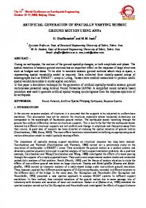
with respect to Vm. There are 42×42 independent grids (1142 wet grids) distributing uniformly over each 3° × 3° study area. 3.1. The first strategy: previous method The first strategy used to defined the value ofαk to adjust the parameter is similar to the work of Fan and Lv [14], that isαk =1.01-0.01k, where k is assimilation step. We analyze the experimental results with the influence radius ranging from 5° to 12° to explore the interference brought by influence radius. When the influence radius is 9°, assimilation results is the most optimal: ME achieves the minimum 0.0038 mmol·N m-1, AAE of Vm drops to 0.0032 day -1 from 0.157 day -1 and RCF is 0.027 after 28 steps (see Table 2). We can see RCF dose not decrease with assimilation steps obviously and fluctuates after 6 steps (see Fig. 3). We attribute this to the improper amount of the modification of parameter because the step-length is very important, and affects the assimilation efficiency and simulative accuracy of simulation. So we design better strategies of optimizing the step-length to improve assimilation efficiency. Table 2. The results of the first strategy Influence radius（°）

ME （mmol·N m-1）

RCF

Vm AAE（day-1）

5

0.0048

0.154

0.045

6

0.0039

0.046

0.032

7

0.0042

0.040

0.034

8

0.0042

0.034

0.033

9

0.0038

0.027

0.033

10

0.0039

0.030

0.033

11

0.0039

0.029

0.035

3.2. The second strategy From Table 2 we can see that the optimal influence radius is 9° when there are 42×42 independent grids in the study area, so 8° and 9° are chosen as influence radius in this section, which reduces times of experiments and provides reference value for real experiments in future. We find the RCF fluctuates regularly after 5 steps whenαk =1, (k=1, 2, 3……28), and five groups of experiments are carried out to compare the simulated results with different αk (see Table 3). The ME, RCF and AAE of Vm all get minimum value in group 3 where αk= (0.7)k-5, k>5, whether the influence radius is 9° or 8°. The RCF is 0.0008 that is 2 orders of magnitude smaller and the ME also reduces to 0.0005 mmol·N m-3 that is 1 order of magnitude smaller than the result of the first strategy mentioned above. The AAE of Vm is 0.021 after assimilation, indicating that the given type of spatially varying Vm is reproduced better. Table 3. Results of the second strategy.

2067

2068 2094

Group of experiment


influence radius is 8°

αk

Vm AAE

ME

（day-1）

（mmol·N m-3）

0.002

0.022

0.0007

0.002

0.022

0.001

0.022

0.0006

0.001

0.021

0.0005

0.0008

0.021

0.0005

0.0009

0.021

0.0007

0.002

0.023

0.0008

0.002

0.023

0.009

0.029

0.0021

0.009

0.028

ME

k